Comparing treatments and finding rates of change

Does chilling reduce carbon dioxide uptake, and does the answer depend on carbon dioxide concentration or plant origin? When does increasing concentration produce the largest increase in uptake? These questions require comparisons of fitted responses and their rates of change, rather than inspection of individual smooths alone. This article uses the same model to answer each question and to explain how the choice of interval changes the conclusion.

The examples use the small CO2 data set distributed with R, plus mgcv, gratia, dplyr and ggplot2. No additional modelling package is needed. We use 2,000 coefficient draws for the illustrated bands and posterior calculations. If a conclusion depends on an interval limit, increase this count and check that the limit is stable.

library("mgcv")
library("gratia")
library("dplyr")
library("ggplot2")

What was measured, and what model is useful?

The R documentation for CO2 describes an experiment on cold tolerance in Echinochloa crus-galli. Uptake was measured at seven concentrations in each of twelve plants, with three plants in each origin and treatment combination. Chilled plants were cooled overnight. The response is uptake in micromoles per square metre per second; conc records ambient concentration in the units supplied with the data (mL/L). These repeated measurements describe curves for individual plants.

plant <- as.data.frame(datasets::CO2)
plant$Plant <- factor(plant$Plant, ordered = FALSE)

uptake_label <- expression(CO[2]~uptake~(mu*mol~m^{-2}~s^{-1}))
concentration_label <- "Ambient CO2 concentration (data units: mL/L)"

ggplot(plant, aes(conc, uptake, colour = Treatment, group = Plant)) +
  geom_point() +
  geom_line(alpha = 0.6) +
  facet_wrap(~ Type) +
  labs(x = concentration_label, y = uptake_label, colour = "Treatment")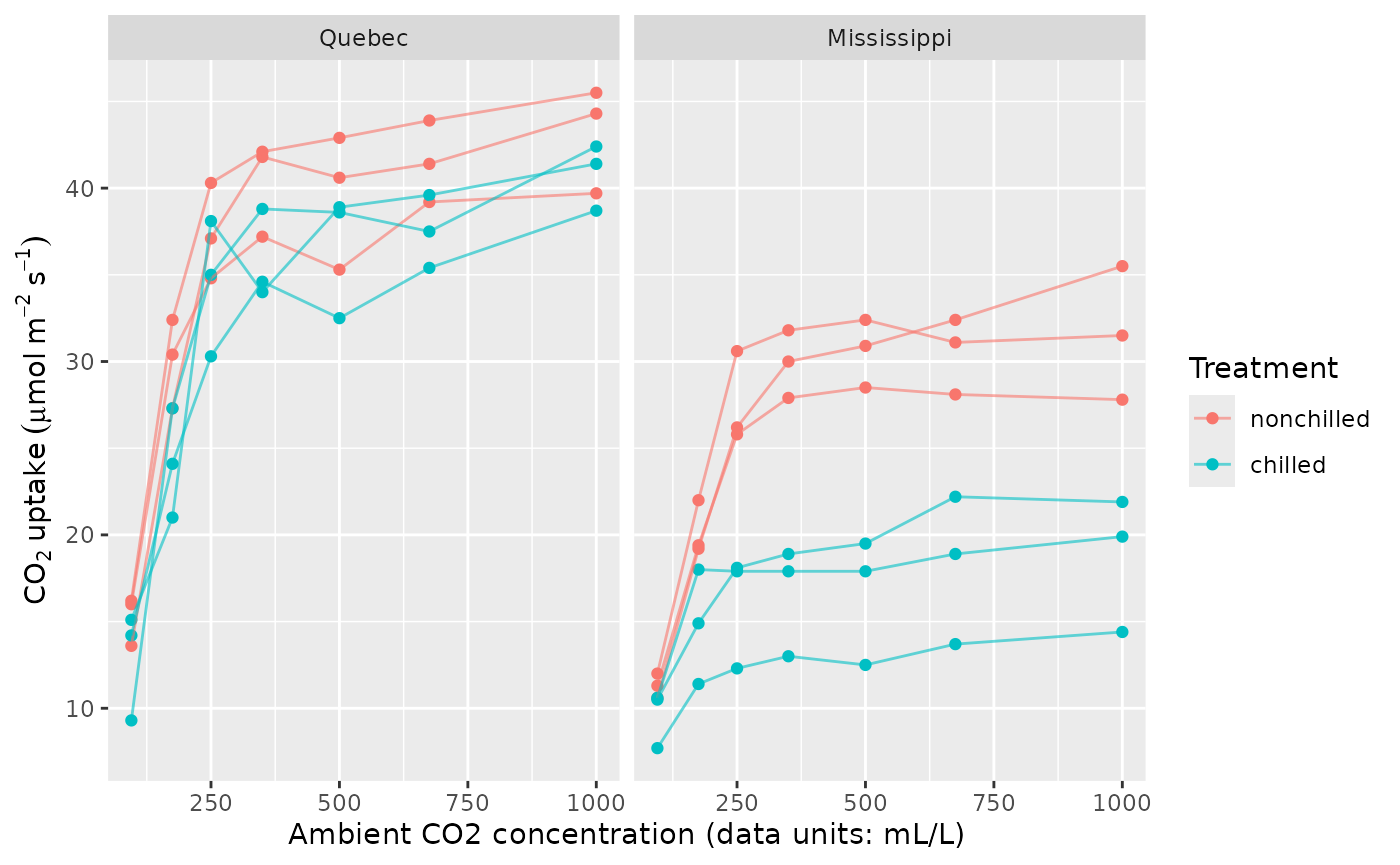

Uptake increases quickly at lower concentrations and then tends to level off. The chilled Mississippi plants have particularly low uptake. We fit a separate smooth concentration response for each treatment, and allow the treatment contrast in average log uptake to differ by origin. A plant random intercept allows measurements from the same plant to share a persistent deviation from the fitted curve.

All responses are positive. A Gamma distribution with a log link preserves positive fitted means and assumes that residual variability grows with the mean. The model assumes that the shape of each treatment curve on the log scale is shared between origins. The origin interaction changes its height. With three plants per combination, sharing those shapes lets us estimate treatment curves without fitting a separate shape to every origin and treatment combination.

m_uptake <- gam(
  uptake ~ Type * Treatment + s(conc, by = Treatment, k = 5) +
    s(Plant, bs = "re"),
  data = plant, family = Gamma(link = "log"), method = "REML"
)
overview(m_uptake)
#> 
#> Generalized Additive Model with 7 terms
#> 
#>   term                             type        k   edf ref.edf statistic p.value
#>   <chr>                            <chr>   <dbl> <dbl>   <dbl>     <dbl> <chr>  
#> 1 Intercept                        parame…    NA  1       1        54.7  < 0.001
#> 2 TypeMississippi                  parame…    NA  1       1        -3.44 0.00102
#> 3 Treatmentchilled                 parame…    NA  1       1        -1.25 0.21582
#> 4 TypeMississippi:Treatmentchilled parame…    NA  1       1        -2.80 0.00668
#> 5 s(conc):Treatmentnonchilled      TPRS        4  3.91    3.99    102.   < 0.001
#> 6 s(conc):Treatmentchilled         TPRS        4  3.88    3.99     69.9  < 0.001
#> 7 s(Plant)                         Random…    12  6.92    8         6.96 < 0.001

k = 5 limits each treatment curve’s complexity; REML estimates the penalties that control its smoothness. It does not force five effective degrees of freedom. The plant intercept accounts for persistent differences in curve height. Residual patterns against concentration can show whether plant differences also involve curve shape; the diagnostic workflow explains checks with fitted effects and simulated effects. The treatment comparison has three independent plants per combination, even though each plant contributes seven measurements.

Compare expected uptake on a supported grid

For each origin and treatment, evaluate concentration across its observed range. .by evaluates expressions within observed groups. This matters when groups have different ranges: using the overall range can extrapolate for some groups. Here the experimental concentration range is the same in all four groups.

uptake_grid <- data_slice(m_uptake,
  conc = evenly(conc, n = 60),
  Plant = level(Plant, as.character(Plant[1])),
  .by = c(Type, Treatment)
)
uptake_grid |>
  group_by(Type, Treatment) |>
  summarise(lower = min(conc), upper = max(conc), .groups = "drop")
#> # A tibble: 4 × 4
#>   Type        Treatment  lower upper
#>   <fct>       <fct>      <dbl> <dbl>
#> 1 Quebec      nonchilled    95  1000
#> 2 Quebec      chilled       95  1000
#> 3 Mississippi nonchilled    95  1000
#> 4 Mississippi chilled       95  1000

The Plant expression supplies one actual plant identifier in each group. We exclude its random effect below, so every curve describes a plant whose random intercept is zero. With a log link, this does not give the mean obtained by averaging over the population distribution of random intercepts. It also excludes measurement noise: the bands concern conditional expected uptake, not future measurements.

uptake_fitted <- fitted_values(m_uptake,
  data = uptake_grid, exclude = "s(Plant)",
  interval = "simultaneous", n_sim = 2000, seed = 2026
)

ggplot(uptake_fitted, aes(conc, .fitted, colour = Treatment, fill = Treatment)) +
  geom_ribbon(aes(ymin = .lower_ci, ymax = .upper_ci), alpha = 0.2,
    colour = NA) +
  geom_line() +
  facet_wrap(~ Type) +
  labs(x = concentration_label, y = uptake_label,
    colour = "Treatment", fill = "Treatment")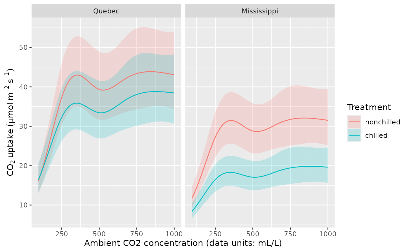

The fitted Mississippi curves are lower, especially after chilling. For the Quebec plants the treatment curves are closer. Overlap between two prediction bands is not a direct test of their difference: both curves depend on the same estimated coefficients, and their errors are correlated.

The default interval = "confidence" gives a separate, pointwise interval at each row. interval = "simultaneous" instead calibrates one band across all 240 supplied rows, including both origins and treatments. It uses the joint coefficient covariance on the link scale and then transforms the limits. Coverage is approximate posterior coverage on this finite grid. It does not extend outside the grid, or guarantee coverage between its points. The returned .se remains a standard error on the link scale.

Estimate the treatment difference directly

conditional_differences() compares whole-model predictions, including the parametric origin and treatment effects. Put Treatment in by and Type in condition to compare treatments within each origin.

treatment_difference <- conditional_differences(m_uptake,
  by = "Treatment", condition = c("conc", "Type"),
  exclude = "s(Plant)", scale = "response",
  uncertainty = "delta", interval = "simultaneous",
  simultaneous_scope = "contrast", n_vals = 60, n_sim = 2000, seed = 2026
)
draw(treatment_difference) +
  labs(x = concentration_label,
    y = "Expected uptake: nonchilled minus chilled")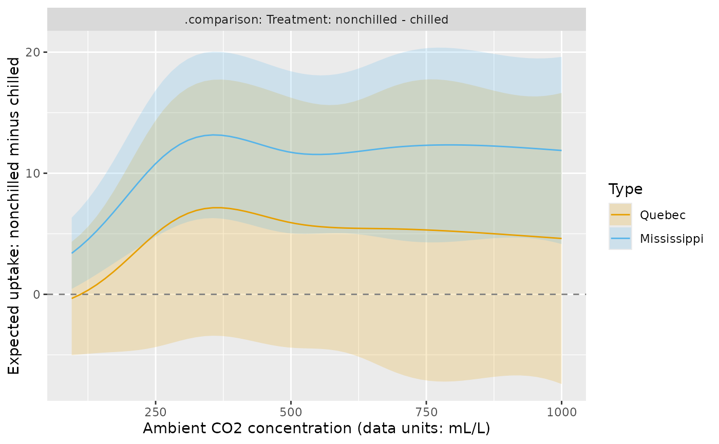

The factor level order determines subtraction: nonchilled minus chilled here. A positive difference means lower uptake after chilling. The Mississippi difference becomes clearly positive over much of the range; the evidence for a difference in Quebec is weaker. The zero reference line and interval limits show which evaluated concentrations support a positive contrast. Where the interval contains zero, the direction of the treatment difference remains unresolved.

The delta method approximates a response-scale difference by its local linear change with the coefficients, then propagates their joint covariance. On the link scale the contrast calculation is linear; on the response scale it is an approximation. Simulation can better describe asymmetric uncertainty after a nonlinear inverse link:

treatment_simulation <- conditional_differences(m_uptake,
  by = "Treatment",
  condition = list(conc = c(250, 500, 750), "Type"),
  exclude = "s(Plant)", scale = "response", uncertainty = "simulation",
  n_sim = 2000, seed = 2026
)
treatment_simulation |>
  select(Type, conc, .level_1, .level_2, .diff, .se, .lower_ci, .upper_ci)
#> # A tibble: 6 × 8
#>   Type         conc .level_1   .level_2 .diff   .se .lower_ci .upper_ci
#>   <fct>       <dbl> <fct>      <fct>    <dbl> <dbl>     <dbl>     <dbl>
#> 1 Quebec        250 nonchilled chilled   5.00  3.45     -1.45      12.1
#> 2 Mississippi   250 nonchilled chilled  10.8   2.17      6.70      15.2
#> 3 Quebec        500 nonchilled chilled   5.92  3.82     -1.42      13.4
#> 4 Mississippi   500 nonchilled chilled  11.7   2.45      7.29      16.7
#> 5 Quebec        750 nonchilled chilled   5.32  4.61     -3.55      14.4
#> 6 Mississippi   750 nonchilled chilled  12.3   2.88      6.60      18.1

For each posterior draw, gratia predicts both treatments with the same coefficient vector and subtracts within that draw. Sampling treatments independently would lose their covariance. These pointwise intervals are equal-tailed posterior quantiles; they need not be symmetric about .diff, which is always the difference of the fitted predictions.

The choice of what is covered jointly matters when comparing more than two groups. Putting both factors in by compares the four joint combinations, giving six pairwise contrasts. simultaneous_scope = "contrast" covers each pair separately across every concentration and conditioning stratum; "all" covers all returned pairs together. Use the latter when the scientific claim concerns any of those six comparisons.

all_differences <- conditional_differences(m_uptake,
  by = c("Type", "Treatment"), condition = "conc", exclude = "s(Plant)",
  uncertainty = "simulation", interval = "simultaneous",
  simultaneous_scope = "all", n_vals = 60, n_sim = 2000, seed = 2026
)
all_differences |>
  group_by(.contrast, Type_1, Treatment_1, Type_2, Treatment_2) |>
  slice_min(abs(conc - 500), n = 1) |>
  ungroup() |>
  select(Type_1, Treatment_1, Type_2, Treatment_2, conc,
    .diff, .lower_ci, .upper_ci)
#> # A tibble: 6 × 8
#>   Type_1      Treatment_1 Type_2     Treatment_2  conc .diff .lower_ci .upper_ci
#>   <fct>       <fct>       <fct>      <fct>       <dbl> <dbl>     <dbl>     <dbl>
#> 1 Quebec      nonchilled  Quebec     chilled      494.  5.97    -5.70       17.6
#> 2 Quebec      nonchilled  Mississip… nonchilled   494. 10.6      0.793      20.4
#> 3 Quebec      nonchilled  Mississip… chilled      494. 22.4     12.7        32.0
#> 4 Quebec      chilled     Mississip… nonchilled   494.  4.61    -5.25       14.5
#> 5 Quebec      chilled     Mississip… chilled      494. 16.4      8.78       24.0
#> 6 Mississippi nonchilled  Mississip… chilled      494. 11.8      4.29       19.3

Simultaneous simulation bands are symmetric calibrated bands about .diff, not equal-tailed pointwise intervals. Both uncertainty methods concern mean differences, not observation noise. They support ordinary single-predictor GAM and BAM families, including Gamma, negative binomial and Tweedie; general families with multiple linear predictors and scam fits are not supported by conditional_differences().

Compare shape separately from complete responses

To ask whether the centred smooth shapes differ, use difference_smooths(). This omits parametric treatment and origin effects by default.

shape_difference <- difference_smooths(m_uptake, select = "s(conc)",
  interval = "simultaneous", n = 60, n_sim = 2000, seed = 2026
)
draw(shape_difference) +
  labs(x = concentration_label, y = "Difference of centred log-uptake smooths")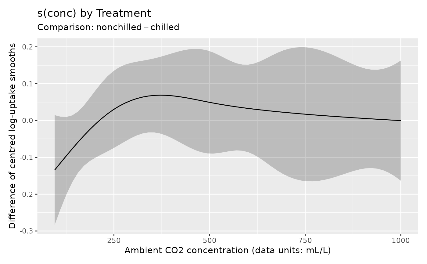

Much of this band contains zero. Thus the marked difference in expected Mississippi uptake need not imply a comparably marked difference in smooth shape. group_means = TRUE can add the means for the smooth’s grouping factor, but for this model the origin-by-treatment interaction makes whole-model conditional_differences() the clearer choice. Smooth differences remain on the link scale, with simultaneous coverage separately for each pair; they do not provide joint coverage across several pairs.

Where does uptake change fastest?

The derivative of expected uptake answers how much uptake changes for a small increase in concentration. This is different from differentiating a centred log-uptake smooth. Hold origin and treatment fixed, and evaluate within the range rather than perturbing an endpoint beyond it.

rate_grid <- data_slice(m_uptake,
  conc = evenly(conc, n = 60, lower = 110, upper = 990),
  Type = level(Type, "Quebec"),
  Treatment = level(Treatment, "nonchilled")
)
rate_delta <- response_derivatives(m_uptake,
  focal = "conc", data = rate_grid, type = "central",
  uncertainty = "delta", exclude = "s(Plant)"
)
rate_simulation <- response_derivatives(m_uptake,
  focal = "conc", data = rate_grid, type = "central",
  uncertainty = "simulation", n_sim = 2000, seed = 2026,
  exclude = "s(Plant)"
)
rates <- bind_rows(delta = rate_delta, simulation = rate_simulation,
  .id = "Uncertainty")
ggplot(rates, aes(conc, .derivative, colour = Uncertainty, fill = Uncertainty)) +
  geom_hline(yintercept = 0, linetype = 2) +
  geom_ribbon(aes(ymin = .lower_ci, ymax = .upper_ci), alpha = 0.15,
    colour = NA) +
  geom_line() +
  labs(x = concentration_label,
    y = "Change in expected uptake per concentration unit")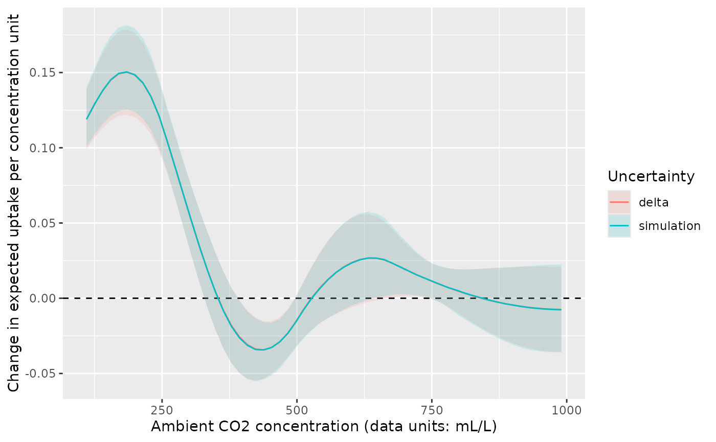

For the nonchilled Quebec curve, the fastest fitted increase is at low concentrations; further increases have a smaller effect over much of the remaining range. The spline also has local decreases: this fit has no monotonicity or asymptote constraint. Near the upper end, intervals include zero, so the estimated small changes have no clearly supported direction.

Both methods return pointwise derivative intervals and .se. Delta uncertainty uses the finite difference of fitted predictions and normal intervals; simulation uses the median and quantiles of derivative draws. The plotted methods agree closely where uncertainty is modest. Differences can grow when the inverse link strongly transforms uncertain coefficients. Delta uncertainty supports single-predictor GAM/BAM families, but does not extend to scam or general families with several predictors; their existing simulation support is unchanged.

The default eps = NULL chooses the perturbation from the fitted covariate range, derivative order and finite-difference method. This reduces dependence on measurement units and avoids many rounding problems in second derivatives. It is a heuristic: near a domain boundary or with unusual scales, supply a positive absolute eps and check stability using nearby values. Set order = 2 to estimate curvature; the first derivative above is the rate of uptake change.

Keep covariate transformations and derivative units distinct

An alternative model uses a smooth of log concentration. This gives more resolution to the lower concentrations where uptake changes quickly. It also assumes a common concentration shape across treatments. We use it to show how a transformed covariate changes the plotting coordinates and derivative units.

m_log_conc <- gam(
  uptake ~ Type * Treatment + s(log(conc), k = 6) + s(Plant, bs = "re"),
  data = plant, family = Gamma(link = "log"), method = "REML"
)
draw(m_log_conc, select = "s(log(conc))", back_transform = TRUE,
  envir = environment()) +
  labs(x = concentration_label, y = "Centred contribution to log uptake")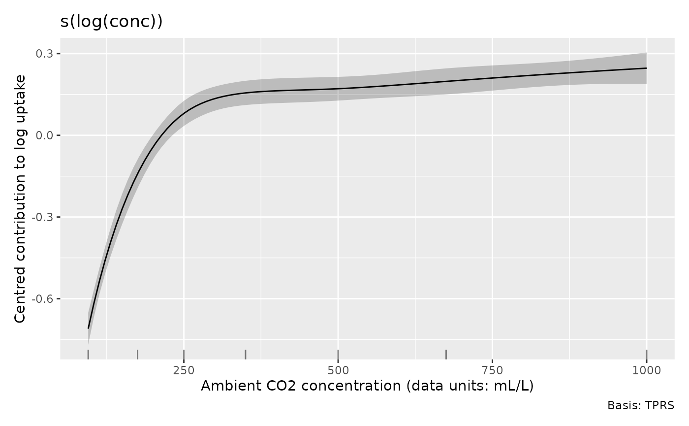

back_transform = TRUE displays concentration in its original units. It changes the horizontal axis, not the meaning of the partial effect on the vertical axis. smooth_estimates(..., back_transform = TRUE) also generates a grid evenly spaced in the raw covariate. The default grid is evenly spaced in log(conc). Supply raw conc values in data for predictions; gratia evaluates the expression.

Here envir = environment() identifies the article’s evaluation environment so the original plant data can be recovered even when the model’s stored formula environment does not locate them. This is useful in notebooks and within fitting functions as well as for custom transformations.

The same coordinate choice applies to parametric effects. For comparison, a model containing a linear log(conc) term assumes a constant log-uptake change per proportional concentration change. It cannot represent the plateau as flexibly as a smooth:

m_log_linear <- gam(
  uptake ~ Type * Treatment + log(conc) + s(Plant, bs = "re"),
  data = plant, family = Gamma(link = "log"), method = "REML"
)
linear_effect <- parametric_effects(m_log_linear, terms = "log(conc)",
  data = rate_grid, envir = environment())
draw(linear_effect, back_transform = TRUE) +
  labs(x = concentration_label, y = "Contribution to log uptake")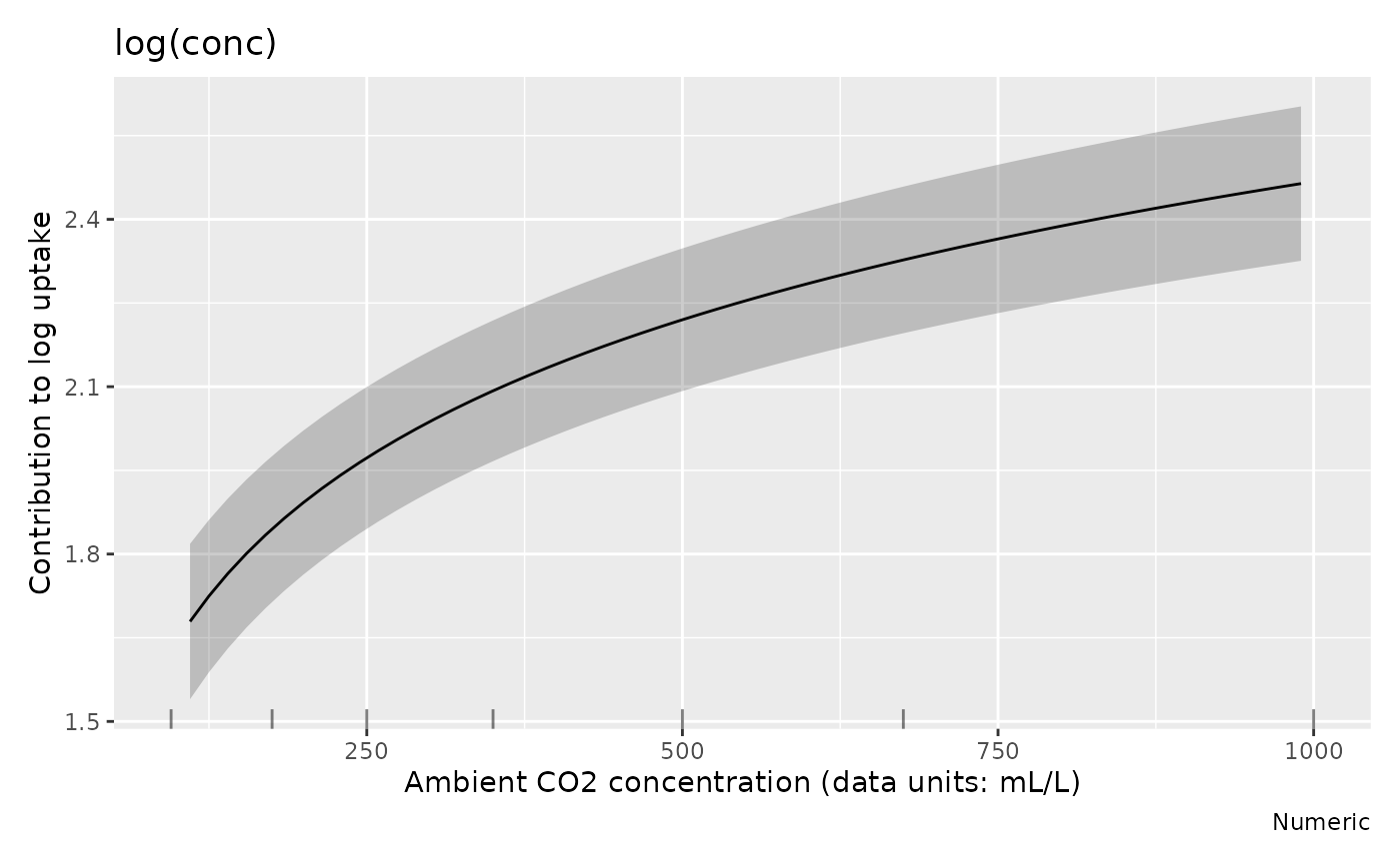

The horizontal axis uses concentration, while the effect remains a contribution to log uptake. Drawing the same object with back_transform = FALSE uses log concentration without changing the estimates. The straight relationship in log concentration appears curved when drawn against concentration in its original units.

log_coordinate_rate <- derivatives(m_log_conc,
  select = "s(log(conc))", data = rate_grid, type = "central"
)
concentration_rate <- derivatives(m_log_conc,
  select = "s(log(conc))", data = rate_grid, type = "central",
  wrt = "covariate"
)
data.frame(conc = rate_grid$conc,
  derivative_per_concentration = concentration_rate$.derivative,
  derivative_per_log_concentration_divided_by_conc =
    log_coordinate_rate$.derivative / rate_grid$conc) |>
  slice(c(1, 20, 40, 60))
#>        conc derivative_per_concentration
#> 1  110.0000                 0.0090013402
#> 20 393.3898                 0.0001036051
#> 40 691.6949                 0.0001670112
#> 60 990.0000                 0.0001294328
#>    derivative_per_log_concentration_divided_by_conc
#> 1                                      0.0090013402
#> 20                                     0.0001036051
#> 40                                     0.0001670112
#> 60                                     0.0001294328

For a smooth contribution f(\log c) the chain rule gives df/dc = (df/d\log c)/c. The two columns agree up to numerical approximation. Both concern the smooth’s contribution to log uptake, not uptake itself. response_derivatives(..., focal = "conc") differentiates complete fitted responses in raw concentration units instead. For tensor smooths such as te(log(conc), temperature), use partial_derivatives() with wrt = "covariate", focal = "conc" while holding temperature fixed. See Functions of covariates and evaluation environments for worked tensor, transformed-offset and local-function examples. Preserve the fitting environment, or pass envir, if expressions need local functions or constants at new data.

Respect the study design when generating predictions

all_levels() is a clearly named alias of evenly() for factors. It keeps their fitted levels, which is useful when deliberately requesting a full factor grid. Such a grid is not always scientifically sensible: each plant in this experiment belongs to only one origin and treatment.

all_levels(plant$Treatment)
#> [1] nonchilled chilled   
#> Levels: nonchilled chilled
observed_plants <- conditional_values(m_uptake,
  condition = c("conc", "Plant", "Treatment", "Type"),
  n_vals = 7, complete = FALSE
)
observed_plants |>
  distinct(Plant, Treatment, Type)
#> # A tibble: 12 × 3
#>    Plant Treatment  Type       
#>    <fct> <fct>      <fct>      
#>  1 Qn1   nonchilled Quebec     
#>  2 Qn2   nonchilled Quebec     
#>  3 Qn3   nonchilled Quebec     
#>  4 Qc1   chilled    Quebec     
#>  5 Qc3   chilled    Quebec     
#>  6 Qc2   chilled    Quebec     
#>  7 Mn3   nonchilled Mississippi
#>  8 Mn2   nonchilled Mississippi
#>  9 Mn1   nonchilled Mississippi
#> 10 Mc2   chilled    Mississippi
#> 11 Mc3   chilled    Mississippi
#> 12 Mc1   chilled    Mississippi

complete = FALSE keeps only the observed combinations of the conditioned factors, here the twelve actual plants with their assigned origin and treatment. It still creates a numeric concentration grid; it does not restrict predictions to measured concentrations, or to a joint region of support for continuous covariates. Include every factor whose combinations need restricting. An omitted factor is still held at its typical value.

fitted_values() reports rows containing combinations of known categorical levels absent from the fitting data. Treat that message as a prompt to examine the prediction design. For example, plant Qn1 was never a chilled Mississippi plant:

hypothetical_grid <- data_slice(m_uptake,
  conc = 500, Type = level(Type, "Mississippi"),
  Treatment = level(Treatment, "chilled"), Plant = level(Plant, "Qn1")
)
fitted_values(m_uptake, data = hypothetical_grid, exclude = "s(Plant)")
#> Prediction data contain 1 row with combinations of categorical predictor levels
#> absent from the fitting data.
#> ℹ Factors: `Type`, `Treatment`, and `Plant`. Input rows: 1.
#> # A tibble: 1 × 9
#>    .row  conc Type        Treatment Plant .fitted    .se .lower_ci .upper_ci
#>   <int> <dbl> <fct>       <fct>     <fct>   <dbl>  <dbl>     <dbl>     <dbl>
#> 1     1   500 Mississippi chilled   Qn1      17.1 0.0730      14.8      19.7

The message checks categorical combinations even when a responsible term is excluded. In the earlier treatment contrast, holding a plant identifier fixed while excluding s(Plant) is intentional: its contribution is zero in both scenarios. When predicting for an observed plant with its random effect included, use that plant’s assigned origin and treatment.

Preserve observation positions when measurements are missing

With na.exclude, results evaluated on the fitting data restore excluded rows as NA. This keeps predictions aligned with the original observation records. For illustration, remove one measured response and refit:

plant_missing <- plant
plant_missing$uptake[1] <- NA_real_
m_missing <- gam(
  uptake ~ Type * Treatment + s(conc, by = Treatment, k = 5) +
    s(Plant, bs = "re"),
  data = plant_missing, family = Gamma(link = "log"), method = "REML",
  na.action = na.exclude
)
fitted_missing <- fitted_values(m_missing)
fitted_missing |>
  mutate(uptake = plant_missing$uptake) |>
  select(.row, conc, uptake, .fitted) |>
  slice_head(n = 3)
#> # A tibble: 3 × 4
#>    .row  conc uptake .fitted
#>   <int> <dbl>  <dbl>   <dbl>
#> 1     1    NA   NA      NA  
#> 2     2   175   30.4    25.5
#> 3     3   250   34.8    35.6

The first observation was excluded from fitting, so its default fitted result is missing. In contrast, explicit prediction data with a missing response can still give a fitted mean when their predictors are present:

prediction_missing <- plant_missing[1:3, ]
prediction_missing$conc[2] <- NA_real_
fitted_values(m_missing, data = prediction_missing) |>
  select(.row, conc, uptake, .fitted)
#> # A tibble: 3 × 4
#>    .row  conc uptake .fitted
#>   <int> <dbl>  <dbl>   <dbl>
#> 1     1    95   NA      15.3
#> 2     2    NA   30.4    NA  
#> 3     3   250   34.8    35.6

The first prediction is available; the second has a missing required predictor and retains its row with an NA result. na.omit retains only fitting rows instead. Partial residuals, fitted/posterior samples and simulations likewise respect na.exclude positions; diagnostic functions align the retained observations before checking their distributions.

Which uncertainty is being propagated?

The examples use mgcv’s approximate Bayesian coefficient covariance, conditional on estimated smoothing parameters. unconditional = TRUE requests the correction for smoothing-parameter uncertainty when it is available. get_vcov() exposes the same matrix for custom calculations:

V <- get_vcov(m_uptake)
dim(V)
#> [1] 24 24
dim(get_vcov(m_uptake, term = "s(conc):Treatmentnonchilled"))
#> [1] 4 4

For APIs that provide frequentist, including difference_smooths(), derivatives() and smooth_estimates(), setting it to TRUE selects the covariance of the penalised coefficient estimators instead. This describes their sampling variability, while the default covariance supplies the approximate posterior intervals used above. get_vcov(..., frequentist = TRUE) gives that matrix, and get_vcov(..., term = "s(conc):Treatmentnonchilled") extracts a term’s coefficient covariance. Keeping the full matrix is essential when comparing two terms whose estimates are correlated.

Distribution parameters and link functions also require explicit choices in models with several predictors. For example, link(gaulss(), parameter = "location") selects the mean’s link, whereas inv_link(gaulss(), parameter = "scale") selects the scale predictor’s inverse link:

link(gaulss(), parameter = "location")(c(1, 2))
#> [1] 1 2
inv_link(gaulss(), parameter = "scale")(c(-1, 0, 1))
#> [1] 2.646347 0.990099 0.366531

The functions follow the fitting package’s parameterisation. As explained in the mgcv gaulss documentation, the second inverse link returns inverse standard deviation, so it should not be labelled standard deviation without taking its reciprocal. These utilities do not remove the multiple-predictor restrictions of the comparison or delta derivative methods.

The fitted model supports lower expected uptake for chilled Mississippi plants over much of the measured range. The Quebec comparison has wider intervals relative to its estimated difference, leaving its direction less clear. For nonchilled Quebec plants, uptake rises fastest at low concentrations and changes more slowly over the remaining range.