Partial derivatives of estimated multivariate smooths via finite differences

Usage

partial_derivatives(object, ...)

# Default S3 method
partial_derivatives(object, ...)

# S3 method for class 'gamm'
partial_derivatives(object, ...)

# S3 method for class 'gam'
partial_derivatives(
  object,
  select = NULL,
  term = deprecated(),
  focal = NULL,
  data = newdata,
  order = 1L,
  type = c("forward", "backward", "central"),
  n = 100,
  eps = 1e-07,
  interval = c("confidence", "simultaneous"),
  n_sim = 10000,
  level = 0.95,
  unconditional = FALSE,
  frequentist = FALSE,
  offset = NULL,
  ncores = 1,
  partial_match = FALSE,
  seed = NULL,
  ...,
  newdata = NULL
)

Arguments

object: an R object to compute derivatives for.
...: arguments passed to other methods.
select: character; vector of one or more smooth terms for which derivatives are required. If missing, derivatives for all smooth terms will be returned. Can be a partial match to a smooth term; see argument partial_match below.
term: Use select instead.
focal: character; name of the focal variable. The partial derivative of the estimated smooth with respect to this variable will be returned. All other variables involved in the smooth will be held at constant. This can be missing if supplying data, in which case, the focal variable will be identified as the one variable that is not constant.
data: a data frame containing the values of the model covariates at which to evaluate the first derivatives of the smooths. If supplied, all but one variable must be held at a constant value.
order: numeric; the order of derivative.
type: character; the type of finite difference used. One of "forward", "backward", or "central".
n: numeric; the number of points to evaluate the derivative at.
eps: numeric; the finite difference.
interval: character; the type of interval to compute. One of "confidence" for point-wise intervals, or "simultaneous" for simultaneous intervals.
n_sim: integer; the number of simulations used in computing the simultaneous intervals.
level: numeric; 0 < level < 1; the confidence level of the point-wise or simultaneous interval. The default is 0.95 for a 95% interval.
unconditional: logical; use smoothness selection-corrected Bayesian covariance matrix?
frequentist: logical; use the frequentist covariance matrix?
offset: numeric; a value to use for any offset term
ncores: number of cores for generating random variables from a multivariate normal distribution. Passed to mvnfast::rmvn(). Parallelization will take place only if OpenMP is supported (but appears to work on Windows with current R).
partial_match: logical; should smooths be selected by partial matches with term? If TRUE, term can only be a single string to match against.
seed: numeric; RNG seed to use.
newdata: Deprecated: use data instead.

Value

A tibble, currently with the following variables:

.smooth: the smooth each row refers to,
.partial_deriv: the estimated partial derivative,
.se: the standard error of the estimated partial derivative,
.crit: the critical value such that derivative ± (crit * se) gives the upper and lower bounds of the requested confidence or simultaneous interval (given level),
.lower_ci: the lower bound of the confidence or simultaneous interval,
.upper_ci: the upper bound of the confidence or simultaneous interval.

Note

partial_derivatives() will ignore any random effect smooths it encounters in object.

Author

Gavin L. Simpson

Examples


library("ggplot2")
library("patchwork")
load_mgcv()
df <- data_sim("eg2", n = 2000, dist = "normal", scale = 0.5, seed = 42)

# fit the GAM (note: for execution time reasons, k is set articifially low)
m <- gam(y ~ te(x, z, k = c(5, 5)), data = df, method = "REML")

# data slice through te(x,z) holding z == 0.4
ds <- data_slice(m, x = evenly(x, n = 100), z = 0.4)

# evaluate te(x,z) at values of x & z
sm <- smooth_estimates(m, select = "te(x,z)", data = ds) |>
  add_confint()

# partial derivatives
pd_x <- partial_derivatives(m, data = ds, type = "central", focal = "x")

# draw te(x,z)
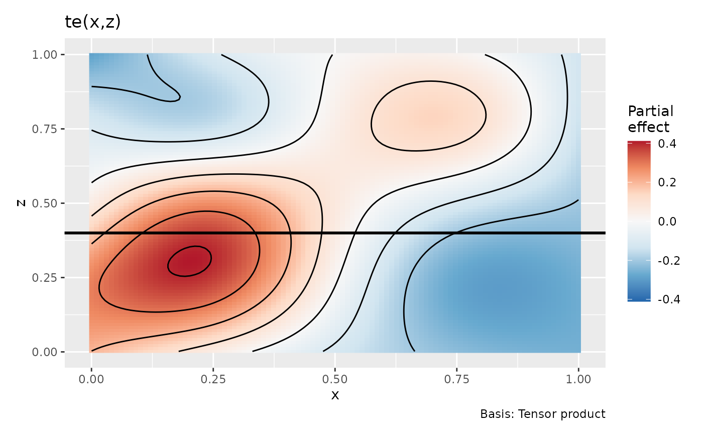
p1 <- draw(m, rug = FALSE) &
  geom_hline(yintercept = 0.4, linewidth = 1)
p1


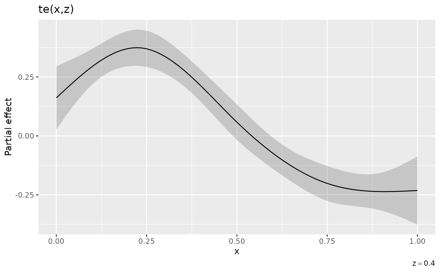
# draw te(x,z) along slice
cap <- expression(z == 0.4)
p2 <- sm |>
  ggplot(aes(x = x, y = .estimate)) +
  geom_ribbon(aes(ymin = .lower_ci, ymax = .upper_ci), alpha = 0.2) +
  geom_line() +
  labs(
    x = "x", y = "Partial effect", title = "te(x,z)",
    caption = cap
  )
p2


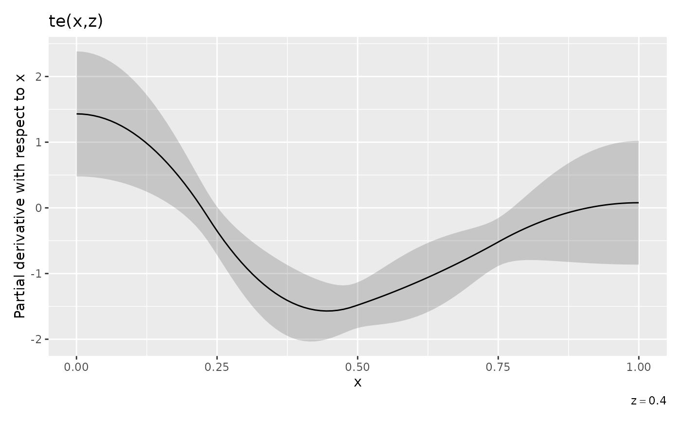
# draw partial derivs
p3 <- pd_x |>
  draw() +
  labs(caption = cap)
p3


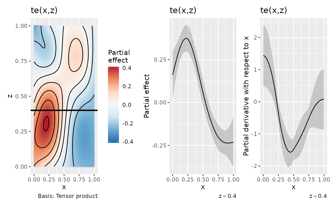
# draw all three panels
p1 + p2 + p3 + plot_layout(ncol = 3)