Differences of factor smooth interactions

Estimates pairwise differences (comparisons) between factor smooth interactions (smooths with a factor by argument) for pairs of groups defined by the factor. The group means can be optionally included in the difference. First and second derivatives of these differences, including partial derivatives across smooth surfaces, can also be estimated.

Usage

difference_smooths(model, ...)

# S3 method for class 'gam'
difference_smooths(
  model,
  select = NULL,
  smooth = deprecated(),
  n = 100,
  n_2d = 50,
  ci_level = 0.95,
  data = NULL,
  group_means = FALSE,
  partial_match = TRUE,
  unconditional = FALSE,
  frequentist = FALSE,
  envir = NULL,
  ...,
  interval = c("confidence", "simultaneous"),
  n_sim = 10000,
  n_cores = 1,
  seed = NULL,
  variables = NULL,
  n_3d = 16,
  n_4d = 4,
  simultaneous_method = c("simulation", "tube"),
  simultaneous_domain = NULL,
  tube_control = list(),
  order = 0L,
  focal = NULL,
  type = c("central", "forward", "backward"),
  eps = NULL,
  wrt = c("smooth", "covariate")
)

# S3 method for class 'scam'
difference_smooths(model, ..., unconditional = FALSE)

Arguments

model

A fitted model.

...

arguments passed to other methods. Not currently used.

select

character, logical, or numeric; which smooths to compare. If NULL, the default, then all model smooths are factor-smooth interactions are compared. Numeric select indexes the smooths in the order they are specified in the formula and stored in object. Character select matches the labels for smooths as shown for example in the output from summary(object). Logical select operates as per numeric select in the order that smooths are stored. Careful selection is needed because it is not allowed to compare smooths of different covariates or of different factor-by variables.

For character select, specific named smooths cane be provided, in which case, the exact names of the smooths (as given by smooths(), for example, can be specified, and partial_match must be set to FALSE.

smooth

Use select instead.

n

numeric; the number of points at which to evaluate the difference between pairs of smooths.

n_2d

numeric; the number of points along each of the first two axes of a smooth surface, including surface panels of higher-dimensional smooths. The default is 50 in plotting and plot-preparation functions. If NULL, use n instead. Ignored when evaluation data are supplied. Factor levels are retained, and curves with only one continuous covariate use n.

ci_level

numeric between 0 and 1; the coverage of credible interval.

data

data frame of locations at which to evaluate the difference between smooths.

group_means

logical; should the group means be included in the difference? Must be FALSE when order > 0.

partial_match

logical; should smooth match partially against smooths? If partial_match = TRUE, smooth must only be a single string, a character vector of length 1. Unlike similar functions, the default here is TRUE because the intention is that users will be matching against factor-by smooth labels.

unconditional

logical; account for smoothness selection in the model?

frequentist

logical; use the frequentist covariance matrix?

envir

an optional environment supplying functions and constants used in model expressions. The available model formula environment is used when NULL. Covariate observations should be supplied in data.

interval

character; "confidence" (the default) gives pointwise intervals. "simultaneous" gives simultaneous intervals for differences of smooths at the supplied covariate combinations, separately for each pair of factor levels.

n_sim

positive integer; number of coefficient draws used for simultaneous intervals. Ignored for pointwise intervals.

n_cores

positive integer; number of cores used by mvnfast::rmvn() for simultaneous intervals. Parallel execution requires OpenMP support.

seed

integer or NULL; optional random seed for simultaneous intervals. An explicit seed preserves the caller's random number state. With NULL, the current random number state is used and advanced.

variables

Character vector giving every covariate of the selected smooths exactly once, in plotting order: x, y, then the conditioning covariate for 3D smooths, or facet rows and columns for 4D smooths. When supplied, selected smooths must use the same covariates. Use fitted coordinate names, such as "log(x)" for a transformed covariate. The default, NULL, favours a two-variable tensor margin for x and y, otherwise retaining fitted order. Grid resolution follows this order. Supplied data are evaluated unchanged. Drawing saved estimates can change the order but uses only points already evaluated; evaluate again to change grid resolution or conditioning values. Continuous covariates must precede factors. Spherical smooths retain their latitude/longitude convention and do not support reordering.

n_3d, n_4d

numeric; the number of conditioning values for smooths of three or four covariates. The defaults are 16 and 4, respectively. If NULL, use n. Ignored when evaluation data are supplied.

simultaneous_method

character; calibration for simultaneous bands. The default, "simulation", uses coefficient draws on the evaluation grid. "tube" uses a conservative Gaussian threshold-crossing bound over a continuous interval for supported one-dimensional cubic splines. See simultaneous_bands.

simultaneous_domain

numeric pair of increasing finite endpoints, or a named list of such pairs keyed by spline coordinate. For tube bands, NULL uses the range of returned evaluation coordinates, including gaps. All returned points must lie inside the interval and the interval must lie inside the fitted spline support. Requires tube calibration.

tube_control

named list controlling numerical tube calibration: rel_tol (default 1e-6), abs_tol (1e-8), subdivisions (1000L), and root_tol (1e-8). Requires tube calibration. Simulation controls n_sim, n_cores (or ncores), and seed are ignored by tube calibration.

order

numeric; 0 (the default) estimates smooth differences; 1 and 2 estimate their first and second derivatives.

focal

character; one differentiation coordinate shared by all compared smooths. Inferred for univariate smooths; required for multivariate smooths when order > 0.

type

character; finite-difference scheme for derivatives. One of "central" (the default), "forward", or "backward".

eps

a positive finite number giving the absolute finite-difference step, or NULL (the default) to choose it automatically. The automatic step is the fitted range of the differentiation coordinate multiplied by .Machine$double.eps^(1 / (order + p)), where p = 2 for central differences and p = 1 for forward or backward differences. A constant coordinate uses its absolute value (or one if zero) instead of its range. The step is rounded upwards and bounded below so that adding it to the coordinates produces a representable change. Stored transformed values or raw covariate summaries supply the range; supplied data are used if neither is available. This is a scale-aware heuristic, not an error bound; unusual function scales or domain boundaries may require explicit eps. For first central differences the two points are separated by eps; for second central differences they are each eps from the target.

wrt

differentiation coordinate: "smooth" (the default) uses the smooth expression, such as log(x); "covariate" uses a raw covariate, such as x, and reevaluates expressions at each finite-difference point.

Value

A tibble of class "difference_smooth". Columns .smooth, .by, .level_1, and .level_2 identify each comparison; .diff contains the estimate for level 1 minus level 2, with .se, .lower_ci, .upper_ci, and evaluation covariates. For order > 0, .diff contains the derivative difference and .focal names its coordinate. The derivative_info attribute records order, focal, wrt, type, and the resolved step eps. The plot_variables attribute records the plotting axes.

Details

With the default simulation calibration, simultaneous intervals cover smooth differences at the evaluated covariate combinations for each pair of factor levels, with approximate posterior probability ci_level when using the Bayesian covariance. They do not provide joint coverage across all pairs, outside the evaluation set, or between its points. With data = NULL, the evaluation set is generated using n, n_2d, n_3d, and n_4d. Differences and interval limits are on the linear predictor scale, including group means when requested. For supported univariate cubic splines, simultaneous_method = "tube" instead covers a continuous interval, including between returned points; see simultaneous_bands. Coverage remains separate for each pair.

variables determines the order used to generate and display the evaluation grid. The first two covariates are the x and y axes. The third covariate defines facets for three-dimensional smooths, or facet rows for four-dimensional smooths; the fourth defines facet columns. Use data to choose particular conditioning values. The resolved order is saved with the estimates for use by draw().

The intervals use the joint coefficient covariance selected by unconditional and frequentist, retaining covariance between the two smooths. The covariance must be positive semidefinite. With frequentist = TRUE, simulation instead uses the frequentist covariance of the coefficient estimators. n_sim, n_cores, and seed are ignored for pointwise intervals. An explicit seed scopes the entire call: each pair uses a new batch of coefficient draws, and the caller's random number state is restored on exit. With seed = NULL, the current random number state is used and advanced.

With order > 0, the estimate is the difference between the derivatives of the selected smooths, on the linear predictor scale. Equivalently, it is the derivative of their difference. The estimate and its uncertainty are computed from the difference of the derivative matrices, retaining covariance between the smooths. Group means are excluded, and tube intervals are unavailable for derivatives; use simulation for simultaneous intervals.

For a multivariate smooth, focal identifies the coordinate to differentiate. All other independent coordinates are fixed at their value in each evaluation row. They can vary between rows, so data may describe a full surface or several slices. order = 2 differentiates twice with respect to focal; mixed partial derivatives are not supported. Generated grids adjust the focal range for the finite-difference scheme; supplied evaluation locations are preserved.

With wrt = "covariate", model expressions are reevaluated after changing the raw focal covariate. Generated raw grids use smooth_data() and require each axis to depend on one distinct original covariate. Supply raw data for other transformations. With wrt = "smooth", only the named smooth coordinate is changed. Derivative controls are ignored when order = 0. Raw-coordinate comparisons match the same original covariates, excluding the comparison factor. Evaluated smooth coordinates may differ between factor levels when a transformation involves that factor. The finite-difference step must fit within the fitted focal range for generated grids, including grids with only one focal value.

Parallel calculation

With mirai and carrier installed, configure workers with mirai::daemons() to distribute calculations across selected smooths. difference_smooths() distributes factor-level comparisons instead. Without configured workers, or with only one calculation, evaluation is serial. These functions leave the caller's worker pool running.

Model selection, evaluation of model expressions and random draws are prepared in the caller. Workers receive the coordinates and coefficient columns needed for their calculation. Custom prediction methods are evaluated in the caller, including custom tensor margins and factor-smooth bases; workers receive their prediction matrices. Simultaneous intervals use successive draws in selection order, so set.seed() gives the same results with or without workers, independently of their number or completion order. derivatives() uses set.seed(); the other functions also accept seed, which restores the caller's random number state on exit.

smooth_samples() draws coefficients jointly once, then reuses those draws for every smooth, preserving dependence and chain identities. Sampling finishes before smooth calculations start, so MH chains and smooth workers are not nested. Sampling thread controls keep their existing meanings. Workers use their configured BLAS thread settings; when using a threaded BLAS, limit its threads before starting daemons to avoid competing threads.

Parallel work is most useful for expensive bases or interval calculations. Small grids can be slower because of transfer and scheduling costs. Large grids and many draws also require memory for worker inputs and returned results, in addition to the final output.

See also

derivatives(), partial_derivatives()

Examples

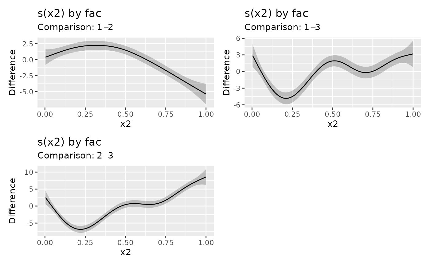
load_mgcv()
# Simulate group-specific curves with Gaussian noise and fit factor-by smooths
df <- data_sim("eg4", n = 300, seed = 42)
m <- gam(y ~ fac + s(x2, by = fac) + s(x0), data = df, method = "REML")

# Compare the centred smooth shapes for each pair of factor levels
sm_dif <- difference_smooths(m, select = "s(x2)")
sm_dif
#> # A tibble: 300 x 9
#>    .smooth .by   .level_1 .level_2 .diff   .se .lower_ci .upper_ci      x2
#>    <chr>   <chr> <chr>    <chr>    <dbl> <dbl>     <dbl>     <dbl>   <dbl>
#>  1 s(x2)   fac   1        2         2.53 0.646      1.26      3.80 0.00359
#>  2 s(x2)   fac   1        2         2.49 0.622      1.27      3.71 0.0136 
#>  3 s(x2)   fac   1        2         2.45 0.598      1.28      3.62 0.0236 
#>  4 s(x2)   fac   1        2         2.41 0.575      1.28      3.54 0.0336 
#>  5 s(x2)   fac   1        2         2.37 0.553      1.29      3.45 0.0435 
#>  6 s(x2)   fac   1        2         2.33 0.531      1.29      3.37 0.0535 
#>  7 s(x2)   fac   1        2         2.29 0.511      1.29      3.29 0.0635 
#>  8 s(x2)   fac   1        2         2.25 0.490      1.29      3.21 0.0735 
#>  9 s(x2)   fac   1        2         2.21 0.471      1.29      3.13 0.0835 
#> 10 s(x2)   fac   1        2         2.17 0.453      1.28      3.06 0.0935 
#> # i 290 more rows
draw(sm_dif)


# Compare rates of change instead of smooth values, using the same fit
slope_dif <- difference_smooths(m, select = "s(x2)", order = 1)
slope_dif
#> # A tibble: 300 x 10
#>    .smooth .focal .by   .level_1 .level_2 .diff   .se .lower_ci .upper_ci
#>    <chr>   <chr>  <chr> <chr>    <chr>    <dbl> <dbl>     <dbl>     <dbl>
#>  1 s(x2)   x2     fac   1        2        -4.03  2.98     -9.88      1.82
#>  2 s(x2)   x2     fac   1        2        -4.03  2.98     -9.88      1.82
#>  3 s(x2)   x2     fac   1        2        -4.03  2.98     -9.86      1.80
#>  4 s(x2)   x2     fac   1        2        -4.03  2.96     -9.82      1.77
#>  5 s(x2)   x2     fac   1        2        -4.03  2.93     -9.76      1.71
#>  6 s(x2)   x2     fac   1        2        -4.02  2.88     -9.68      1.63
#>  7 s(x2)   x2     fac   1        2        -4.02  2.83     -9.58      1.54
#>  8 s(x2)   x2     fac   1        2        -4.02  2.78     -9.46      1.43
#>  9 s(x2)   x2     fac   1        2        -4.01  2.72     -9.34      1.31
#> 10 s(x2)   x2     fac   1        2        -4.01  2.66     -9.21      1.20
#> # i 290 more rows
#> # i 1 more variable: x2 <dbl>