Intervals for shape-constrained smooths • gratia

A fitted increasing or convex smooth can have interval endpoints that lack the fitted shape. gratia provides two ways to use shape restrictions in uncertainty calculations: transform the endpoints of an initial band, or retain an explicit set of admissible coefficient vectors. These answer different questions. The first supplies shaped endpoint curves on an evaluation grid; the second describes whole functions satisfying coefficient restrictions, including equalities.

library("mgcv")
library("gratia")
library("ggplot2")

Shape enforcement and initial uncertainty

shape_intervals() accepts estimates and existing endpoints independently of any model. It first applies a zero lower bound when requested, then sorts values along each monotone coordinate, then takes the greatest convex minorant along one curvature coordinate. The greatest convex minorant is the largest convex curve lying below the supplied values. Concavity uses its negative counterpart. This follows the operator approach of Chen and colleagues (2021), building on monotone rearrangement.

x <- c(0, 0.1, 0.35, 0.7, 1)
estimate <- c(0.1, 0.3, 0.2, 0.8, 1.1)
shaped <- shape_intervals(
  estimate, estimate - 0.3, estimate + 0.3,
  data = data.frame(x = x), constraints = list(x = c("m+", "c+")),
  interval = "simultaneous", level = 0.95
)
shaped
#> # A tibble: 5 × 4
#>       x .estimate .lower_ci .upper_ci
#>   <dbl>     <dbl>     <dbl>     <dbl>
#> 1  0        0.1      -0.2       0.4  
#> 2  0.1      0.157    -0.143     0.457
#> 3  0.35     0.3       0         0.6  
#> 4  0.7      0.731     0.431     1.03 
#> 5  1        1.1       0.8       1.4
attr(shaped, "interval_info")
#> $method
#> [1] "shape"
#> 
#> $level
#> [1] 0.95
#> 
#> $interval
#> [1] "simultaneous"
#> 
#> $source
#> [1] "supplied"
#> 
#> $correction
#> [1] "none"
#> 
#> $shape
#> $shape$x
#> [1] "m+" "c+"
#> 
#> 
#> $operator
#> [1] "range, rearrangement, directional convex minorant"
#> 
#> $domain
#> [1] "evaluation grid"
#> 
#> $scope
#> [1] "grid"
#> 
#> $coverage
#> [1] "whole-grid containment preserved"
#> 
#> $pointwise_calibration
#> [1] "not requested"
#> 
#> $interpretation
#> [1] "inherited from input"

The interval type and level describe the supplied band; this illustrative input has no statistical calibration. The returned table contains .estimate, .lower_ci and .upper_ci, with method information in interval_info.

The supported codes are "+" for nonnegative values, "m+" and "m-" for increasing and decreasing values, and "c+" and "c-" for convexity and concavity. Increasing and decreasing include flat sections. A complete Cartesian grid can have monotonicity in several directions and curvature in at most one direction. These are directional restrictions: convexity along one coordinate does not establish joint convexity of a surface.

Rows may be unordered and coordinates may be irregularly spaced. Convexity uses slopes computed from actual coordinate differences. Sorting assigns equal mass to each distinct grid coordinate; on an irregular grid this is an empirical rearrangement, with no claim about distance measured uniformly across the coordinate domain. Duplicate grid rows and incomplete product grids are rejected.

What the transformation guarantees

Write T for the complete shape operator and f for target values satisfying the requested shape on the grid. The operator preserves order and fixes f. Consequently,

L \leq f \leq U \quad\Longrightarrow\quad T(L) \leq T(f)=f \leq T(U),

where each inequality holds at every grid point together. Thus every instance in which the initial band covers the entire grid remains covered after transformation. The maximum width over the grid cannot increase, although the width at an individual point can increase.

This implication does not establish nominal coverage for the initial band. In particular, transforming separately calibrated pointwise limits does not preserve their marginal coverage at each point: sorting moves information between coordinates. interval = "pointwise" records this source calibration without assigning new pointwise coverage to the result. Penalization bias or an inadequate covariance approximation can also affect initial coverage; the shape operation does not correct either problem.

The coverage statement concerns the evaluation grid. Connecting the returned points by straight lines preserves the named curve shapes, but does not extend coverage to every point between them. Nor do the transformed values necessarily represent a spline in the original fitted basis or satisfy its centring equalities.

What the validation simulations showed

The reproducible experiment in notes/scasm/shape-coverage.R separates known-variance Gaussian calibration from fitted scasm uncertainty. It uses 2,000 repetitions per known-Gaussian scenario and 400 attempted fits per scasm scenario, including exactly flat and exactly linear truths. At 95% coverage, the binomial Monte Carlo standard error is about 0.5 percentage points for 2,000 repetitions and 1.1 percentage points for 400 successful fits. The scasm experiment applies the low-level operator to fitted response curves including their intercepts, giving each simulated truth a fixed reference level.

For a nearly flat increasing truth, the smallest marginal coverage over grid points fell from 93.65% to 38.00% after transforming Gaussian pointwise limits. Using an initially calibrated simultaneous band, whole-grid coverage instead changed from 94.85% to 95.75%. No originally covering whole-grid band lost coverage in any of the 49,182 paired transformations across the experiment. These are empirical checks of the event-inclusion result, rather than a reason to interpret transformed pointwise limits as calibrated intervals.

The scasm examples also show that shape enforcement retains limitations of the initial uncertainty. For a nearly binding increasing, convex truth, the transformed Gaussian simultaneous band covered the whole grid in 313 of 342 returned fits: 91.52%, with Monte Carlo standard error 1.51 percentage points. The other 58 attempts raised upstream fitting errors, so this estimate is conditional on a model being returned. The saved reports record all errors and warnings and distinguish them from interval calculations. Comparing selected smoothing with a small fixed penalty also changed local bias. The small-penalty comparison records estimates only; it does not assess interval width or separate smoothing bias from the effects of a finite spline basis and binding restrictions. Enforcing shape supplies no additional correction for smoothing bias.

An increasing, convex scasm smooth

For supported mgcv::scasm() components, select the transformation explicitly with interval_method = "shape". The default initial source is Gaussian: shape_source = "gaussian". Existing interval defaults are unchanged.

set.seed(1701)
d <- data.frame(x = runif(200))
d$y <- 2 * d$x + 4 * d$x^2 + rnorm(nrow(d), sd = 0.2)
m <- scasm(
  y ~ s(x, bs = "sc", xt = c("m+", "c+"), k = 6),
  data = d, bs = 0
)
curve <- smooth_estimates(
  m, select = "s(x)", interval = "simultaneous",
  interval_method = "shape", shape_source = "gaussian",
  n = 100, n_sim = 2000, seed = 1702
)
draw(curve)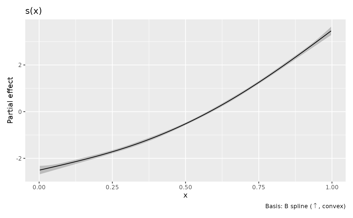

This displays the smooth component on its model scale. The intercept is not added. scasm components use component-only uncertainty by default; an explicit request for overall_uncertainty = TRUE is rejected for shape intervals. Arbitrary effect shifts and transformations are also rejected, because they can change the asserted shape. Standard errors retained in the result describe the initial uncertainty calculation; transformed endpoints are not reconstructed from a standard error and a Gaussian critical value.

Default plot captions show the basis and named shapes. The interval source, level and coverage information remain in the result’s interval_info attribute and in this documentation.

By default the Gaussian source uses the model’s approximate Bayesian covariance. frequentist = TRUE instead requests the frequentist covariance. Neither choice constructs a posterior restricted to the feasible coefficient space. An interpretation as posterior probability requires an initially calibrated posterior region and a posterior supported on the stated shapes. unconditional retains its existing meaning for the initial covariance calculation, including the model’s availability of smoothing-parameter uncertainty corrections; it adds no new calibration to shape enforcement.

The same method selection is available through draw(), assemble() and confint() for supported smooth components. For example, draw(m, interval = "simultaneous", interval_method = "shape", n_sim = 2000, seed = 1702) computes and displays the intervals in one call. Select only eligible terms: every selected smooth must have named restrictions actually retained by the fitted model. General coefficient constraints belong in an explicit set, as described below. Numeric by variables are unsupported, because multiplying a component by a varying value changes its shape.

General pc inequalities can replace the named coefficient restrictions in mgcv while leaving the original xt request in the fitted object. Captions identify that request as not retained, and automatic shape intervals reject it. Ordinary point equalities that leave the named inequalities intact are supported. Derivative-valued bases are rejected: their values do not inherit the named shape of the original spline.

For transformed covariates, shape is asserted in the coordinates used by the model. For example, a restriction on s(log(x), ...) concerns log(x); curvature in that coordinate need not be curvature in x.

A tensor with a constrained direction

Tensor restrictions require particular care: retained coefficient inequalities alone do not imply the named shape when complementary basis functions can be negative. Automatic shape inference therefore accepts unreparameterized univariate B-spline margins, fitted with np = FALSE, within their basis domains. Both "sc" and ordinary "bs" margins can be used in this supported construction.

set.seed(1703)
surface_data <- data.frame(x = runif(300), z = runif(300))
surface_data$y <- exp(1.5 * surface_data$x) + surface_data$z^2 +
  rnorm(nrow(surface_data), sd = 0.15)
surface_model <- scasm(
  y ~ te(x, z, bs = c("sc", "bs"), k = c(5, 5),
    xt = list("m+", NULL), np = FALSE),
  data = surface_data, bs = 0
)
surface <- smooth_estimates(
  surface_model, select = "te(x,z)", interval = "simultaneous",
  interval_method = "shape", n_2d = 30, dist = 0,
  n_sim = 2000, seed = 1704
)
draw(surface)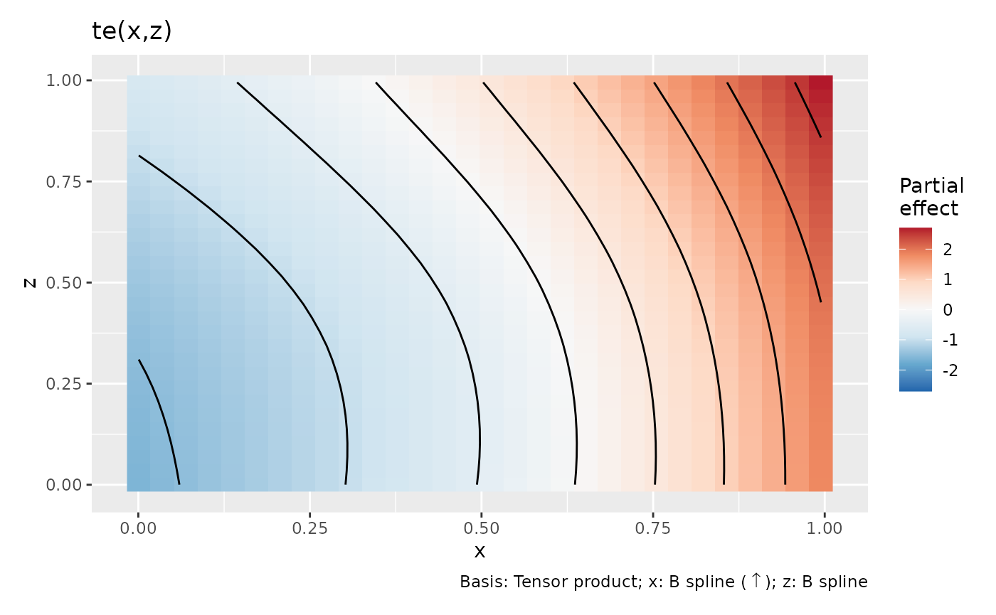

The surface and its endpoints increase with x at fixed z; no restriction is imposed in z. dist = 0 retains the complete product grid needed by the operator. Removing points distant from observations would leave missing slices. Evaluation outside the fitted B-spline domains is rejected.

Automatic curvature inference additionally requires regular knots and a sufficient spline degree. In mgcv 1.9-4, the raw second coefficient differences used by "c+" and "c-" do not ensure spline curvature with arbitrary irregular knots. Equal spacing is checked to rounding precision, because even small departures can reverse curvature when a coefficient restriction binds. Requests with those knots are rejected. The low-level operator can still enforce a justified shape directly on an irregular evaluation grid; that is a separate statement from the shape implied by fitted inequalities. Requests for multiple curvature directions are also rejected because a later convexification can destroy curvature enforced in an earlier direction.

How this differs from stored bootstrap limits

With bs > 0, a scasm fit stores feasible bootstrap coefficient columns in model$bs. Its bootstrap holds smoothing parameters fixed and perturbs a final working likelihood problem. Native intervals evaluate those columns, take pointwise percentiles and, when svar.only is present, adjust endpoints using the mean difference between Bayesian and frequentist standard errors. Percentiles of convex functions need not be convex, and the endpoint adjustment can alter restrictions further.

interval_method = "shape", shape_source = "bootstrap" applies the same shape operators to these native pointwise limits. It requires valid stored draws; simultaneous bootstrap bands remain unsupported. No additional bias correction is introduced. This source requires frequentist = FALSE and unconditional = FALSE, matching the stored draws and native correction. Feasibility of the draws does not establish coverage of their percentiles: Andrews (2000) shows that bootstrap calibration can fail at parameter boundaries. Applying a shape operator preserves whole-grid coverage events already present, without repairing their probability.

Equalities and coupled coefficient restrictions

An integral equality cannot generally be assigned to two different ordered endpoint curves. If both have integral one and their difference is nonnegative, that difference must have integral zero. A useful uncertainty description instead retains a set of whole functions.

shape_confidence_set() stores the intersection

\{b: L\leq Xb\leq U,\quad A_{\mathrm{in}}b\geq b_{\mathrm{in}}, \quad Cb=d\}.

Here is a three-coefficient example representing the values of a piecewise linear curve at x = c(0, 0.5, 1). The positive weights below give its exact integral over [0, 1], which is required to equal one. A spline analysis would supply its own prediction matrix and integrals of basis functions.

weights <- c(0.25, 0.5, 0.25)
region <- shape_confidence_set(
  X = diag(3), lower = c(0, 0, 0), upper = c(2, 2, 2),
  Ain = diag(3),
  C = matrix(weights, nrow = 1), d = 1,
  level = 0.95, interpretation = "confidence", band_type = "simultaneous"
)
in_shape_set(region, c(0.5, 1, 1.5))
#> [1] TRUE
in_shape_set(region, c(0.5, 1, 1))
#> [1] FALSE

The level and band type again record the caller’s calibration. On a feasible true coefficient vector, intersection preserves exactly the initial band’s coverage event. Pointwise limits alone do not provide a simultaneous region. in_shape_set() checks candidate vectors with a documented absolute tolerance; it neither samples the set nor optimizes over it. Construction does not test whether the restrictions define an empty set. Coordinatewise extrema of the set need not themselves satisfy its equalities.

The set representation supports linear equalities and coupled inequalities without replacing them by shaped endpoints. Ellipsoidal initial regions, optimization of bounds over the admissible set and constrained posterior sampling are separate extensions. A Bayesian sampler would need to specify and sample a posterior supported on the coefficient restrictions; see Hazelton and Turlach (2011) for shape-constrained penalized splines. Likewise, Dümbgen (2003) constructs calibrated bands using multiscale tests in a Gaussian white-noise model. Those calibration results are distinct from the finite-grid endpoint transformation implemented here.