Functions of covariates and evaluation environments • gratia

A smooth can depend on a function of a covariate rather than on the raw covariate. The same distinction arises with offsets, such as logged effort in a count model.

set.seed(42)
dat <- data.frame(x = runif(150, 1, 5), effort = runif(150, 1, 3))
dat$y <- rpois(nrow(dat), dat$effort * exp(sin(log(dat$x))))
m <- gam(y ~ s(log(x), k = 6) + offset(log(effort)),
  family = poisson(), data = dat, method = "REML")

Raw data and smooth coordinates

Supply raw covariates to evaluate the model at new observations. Gratia computes log(x) and, for full predictions, offset(log(effort)). An isolated smooth does not require unrelated predictors or the model offset.

nd <- data.frame(x = seq(1.2, 4.8, length.out = 8), effort = 2)
smooth_estimates(m, data = nd["x"])
#> # A tibble: 8 × 7
#>   .smooth   .type .by   .estimate    .se `log(x)` .gratia_raw_x
#>   <chr>     <chr> <chr>     <dbl>  <dbl>    <dbl>         <dbl>
#> 1 s(log(x)) TPRS  NA      -0.544  0.107     0.182          1.2 
#> 2 s(log(x)) TPRS  NA      -0.323  0.0748    0.539          1.71
#> 3 s(log(x)) TPRS  NA      -0.160  0.0543    0.801          2.23
#> 4 s(log(x)) TPRS  NA      -0.0318 0.0428    1.01           2.74
#> 5 s(log(x)) TPRS  NA       0.0747 0.0396    1.18           3.26
#> 6 s(log(x)) TPRS  NA       0.166  0.0425    1.33           3.77
#> 7 s(log(x)) TPRS  NA       0.245  0.0487    1.46           4.29
#> 8 s(log(x)) TPRS  NA       0.315  0.0561    1.57           4.8
fitted_values(m, data = nd)
#> # A tibble: 8 × 7
#>    .row     x effort .fitted    .se .lower_ci .upper_ci
#>   <int> <dbl>  <dbl>   <dbl>  <dbl>     <dbl>     <dbl>
#> 1     1  1.2       2    2.51 0.107       2.03      3.09
#> 2     2  1.71      2    3.13 0.0748      2.70      3.62
#> 3     3  2.23      2    3.68 0.0543      3.31      4.09
#> 4     4  2.74      2    4.18 0.0428      3.85      4.55
#> 5     5  3.26      2    4.65 0.0396      4.31      5.03
#> 6     6  3.77      2    5.10 0.0425      4.69      5.54
#> 7     7  4.29      2    5.52 0.0487      5.01      6.07
#> 8     8  4.8       2    5.92 0.0561      5.30      6.61

Automatic smooth grids are evenly spaced in the smooth coordinate, here log(x), and the output and plot axes use that name. They use stored evaluated covariates, so they do not need to reconstruct an inverse transformation.

sm <- smooth_estimates(m, n = 30)
draw(sm)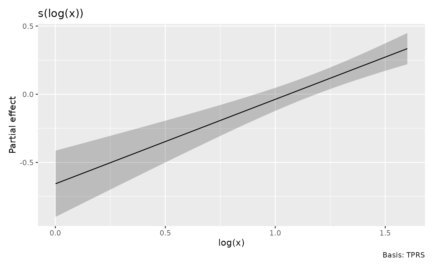

An explicitly evaluated column is also accepted:

evaluated <- data.frame(`log(x)` = log(nd$x), check.names = FALSE)
smooth_estimates(m, data = evaluated)
#> # A tibble: 8 × 6
#>   .smooth   .type .by   .estimate    .se `log(x)`
#>   <chr>     <chr> <chr>     <dbl>  <dbl>    <dbl>
#> 1 s(log(x)) TPRS  NA      -0.544  0.107     0.182
#> 2 s(log(x)) TPRS  NA      -0.323  0.0748    0.539
#> 3 s(log(x)) TPRS  NA      -0.160  0.0543    0.801
#> 4 s(log(x)) TPRS  NA      -0.0318 0.0428    1.01 
#> 5 s(log(x)) TPRS  NA       0.0747 0.0396    1.18 
#> 6 s(log(x)) TPRS  NA       0.166  0.0425    1.33 
#> 7 s(log(x)) TPRS  NA       0.245  0.0487    1.46 
#> 8 s(log(x)) TPRS  NA       0.315  0.0561    1.57

If raw inputs and evaluated columns are both supplied, expressions are recomputed from the raw inputs. Stored model frames and automatically prepared grids retain their evaluated coordinates.

data_slice() works with raw variables. Supply reference data if the original raw covariates cannot be recovered; transformed values are not renamed as raw variables or automatically inverted.

data_slice(m, x = evenly(x, n = 8), effort = 2, data = dat)
#> # A tibble: 8 × 2
#>       x effort
#>   <dbl>  <dbl>
#> 1  1.00      2
#> 2  1.57      2
#> 3  2.13      2
#> 4  2.70      2
#> 5  3.26      2
#> 6  3.83      2
#> 7  4.39      2
#> 8  4.96      2

Choosing the plotted covariate scale

Drawing methods use the model’s covariate coordinates by default. For example, log(x) is plotted against log(x), with a matching axis label, whether it is inside a smooth or a parametric term. Set back_transform = TRUE to display x instead. This changes the plotting coordinates and labels; the estimated partial effect and its interval keep their meaning. Use fun to transform the partial effect itself.

draw(m, back_transform = TRUE)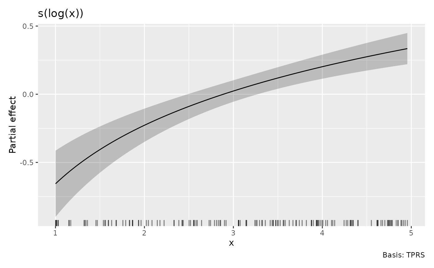

sm_raw <- smooth_estimates(m, back_transform = TRUE)
draw(sm_raw, back_transform = TRUE)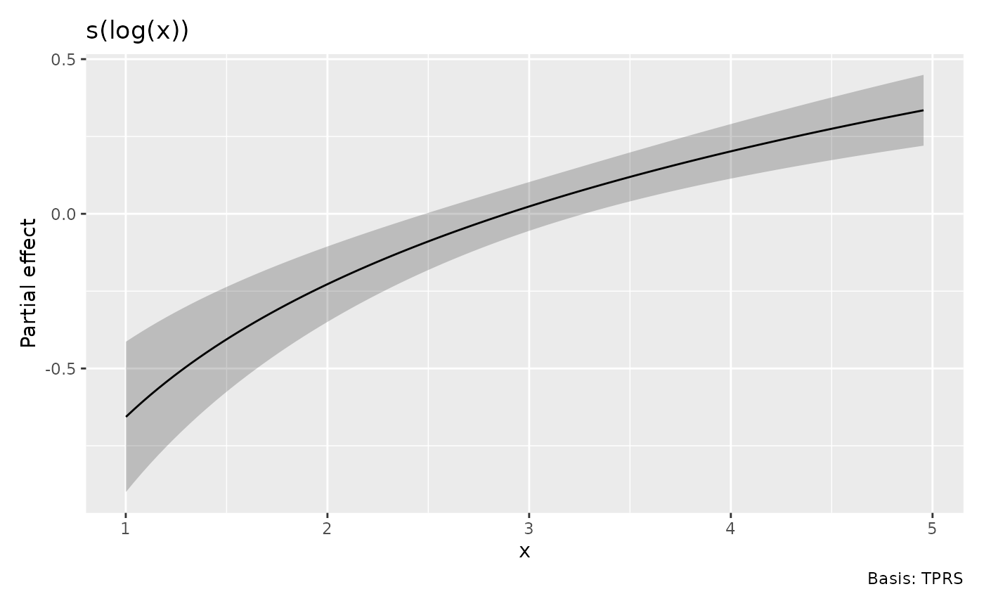


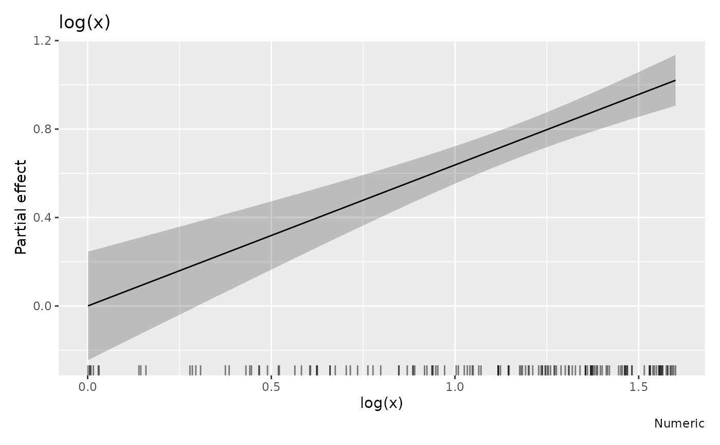
m_parametric <- gam(y ~ log(x), family = poisson(), data = dat)
draw(m_parametric)

draw(m_parametric, back_transform = TRUE)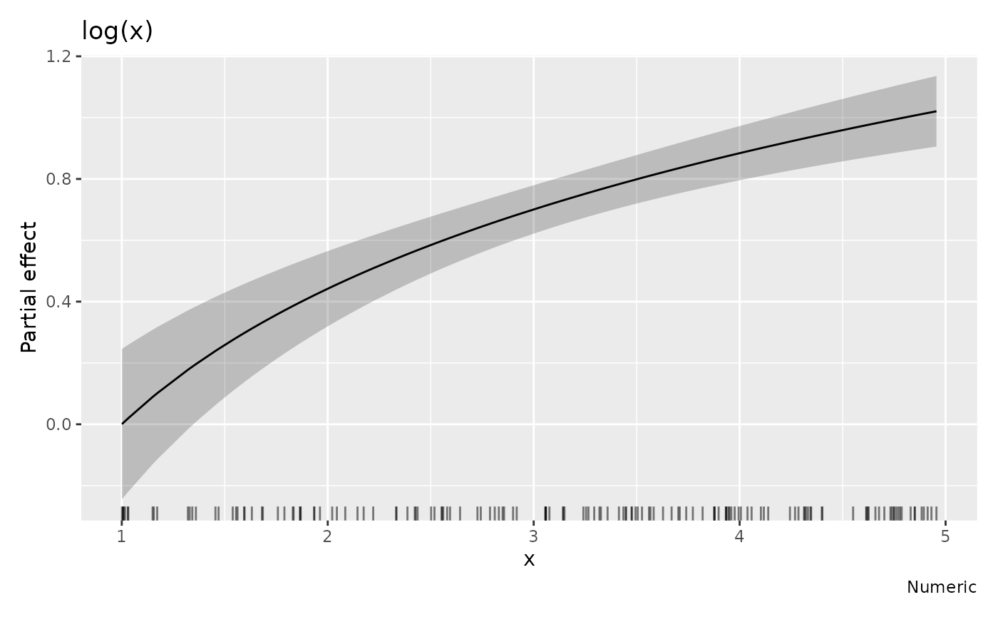

pe <- parametric_effects(m_parametric)
draw(pe, back_transform = TRUE)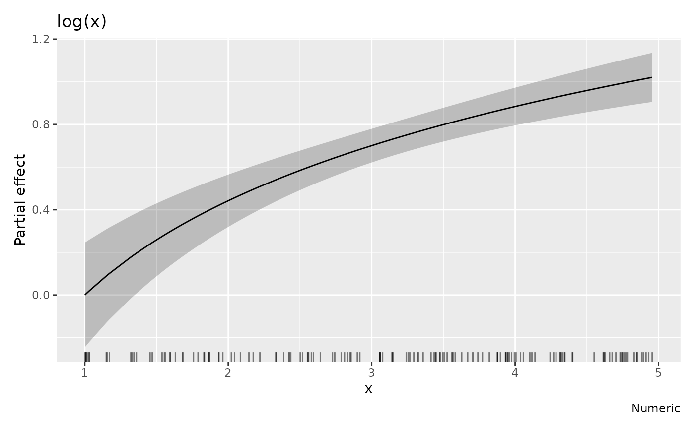

The same rule applies to each covariate in tensor products and parametric interactions, including covariates used for conditioning facets. Rugs and partial-residual locations follow the displayed scale. Surface coordinates can become irregularly spaced after changing scale; these plots use rectangles bounded by adjacent coordinate midpoints to avoid shifting raster pixels.

dat_surface <- transform(dat, z = runif(nrow(dat), 1, 4))
m_surface <- gam(y ~ te(log(x), sqrt(z)), family = poisson(),
  data = dat_surface, method = "REML")
draw(m_surface, back_transform = TRUE, contour = FALSE)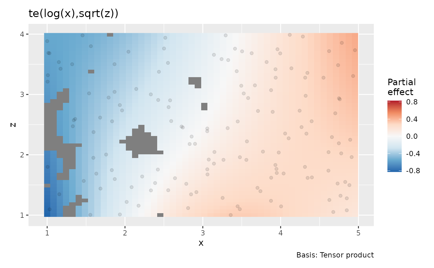

Smooth grids are evenly spaced on the model scale by default. For example, three points for s(log(x)) with x ranging from 1 to 100 correspond to raw values 1, 10, and 100. With smooth_estimates(..., back_transform = TRUE), the grid is evenly spaced in raw x: 1, 50.5, and 100. The expressions are then evaluated forwards and estimates computed at those points. draw(m, back_transform = TRUE) performs this preparation automatically.

Precomputed estimates retain their chosen evaluation points. An object created on a transformed-only grid cannot be drawn on the original scale: its raw coordinates are unavailable. Recompute it with back_transform = TRUE, or supply raw prediction rows through data. Returned estimates retain model coordinates and auxiliary .gratia_raw_* columns, so either drawing scale can be selected without changing the estimates. Subsets and confidence intervals retain these coordinates.

There is no list of supported inverse functions. Each smooth axis must depend on one distinct original model covariate, and gratia must be able to recover that covariate and evaluate the expression. For example:

foo <- sqrt
m_foo <- gam(y ~ s(foo(x), k = 6), family = poisson(), data = dat)
sm_foo <- smooth_estimates(m_foo, back_transform = TRUE, envir = environment())
draw(sm_foo, back_transform = TRUE)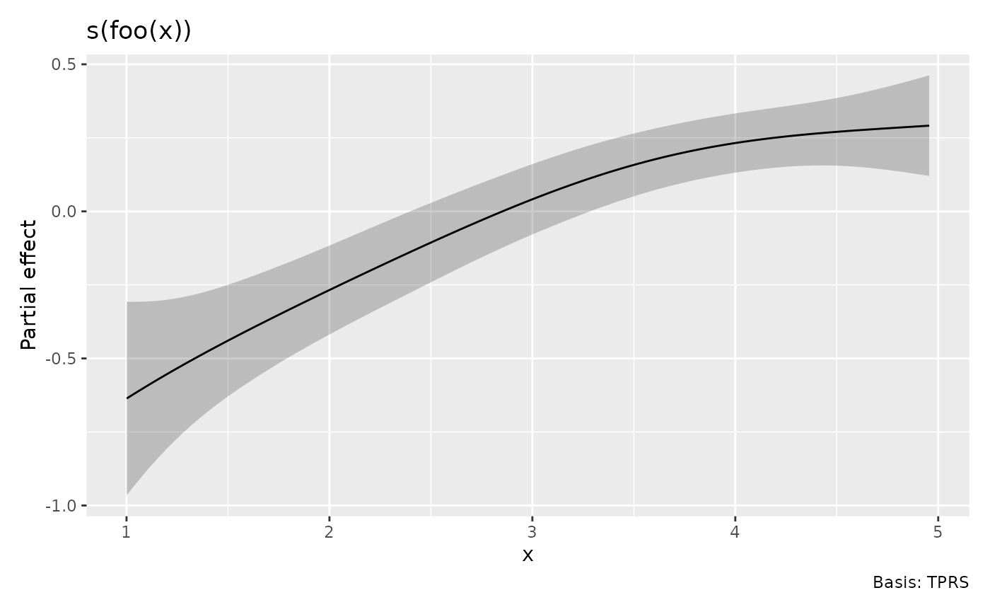

Raw fitting rows are recovered and checked against the stored fitting observations. If the fitting data are unavailable, or changed functions or constants no longer reproduce the fit, recovery fails. Supply raw prediction rows in data and functions or constants in envir as needed. Already prepared estimates can be drawn without recovering data or evaluating functions again. When prediction data are supplied, unavailable raw fitting observations omit rugs and partial residuals. Prediction rows are not substituted for observed data. envir is used for both predictions and observation recovery.

Typical values added by smooth_data(..., include_all = TRUE) do not identify the original coordinates of a model-scale grid. Prepare that grid with back_transform = TRUE to retain raw axes. For numeric by smooths, automatic grids evaluate the smooth with multiplier one, even for s(log(x), by = x); the original axis is retained separately. Supplied raw prediction rows use their actual by values.

Soap-film boundary coordinates are stored on the model scale. A transformed boundary has no retained raw coordinates, so raw-scale drawing raises an error. Draw these soap films with back_transform = FALSE to retain their boundaries.

Parametric effects likewise retain both coordinate scales by row, including for many-to-one functions. Multi-column basis terms such as poly(x, 2) and parametric expressions with no single coordinate per input retain raw axes.

The old parametric_effects(transform = ...) argument is deprecated. Replace transform = TRUE with back_transform = FALSE, and transform = FALSE with back_transform = TRUE.

Local functions

A fitted model may retain the formula expression without retaining the local environment in which it was evaluated. Preserve that environment when fitting if you will need a local function at new observations.

fit_local <- function(dat) {
  shift <- 0.5
  transform_x <- function(x) log(x + shift)
  f <- y ~ s(transform_x(x), k = 6) + offset(log(effort))
  list(model = gam(f, family = poisson(), data = dat, method = "REML"),
    envir = environment(f))
}
bundle <- fit_local(dat)
smooth_estimates(bundle$model, data = nd, envir = bundle$envir)
#> # A tibble: 8 × 7
#>   .smooth           .type .by   .estimate    .se `transform_x(x)` .gratia_raw_x
#>   <chr>             <chr> <chr>     <dbl>  <dbl>            <dbl>         <dbl>
#> 1 s(transform_x(x)) TPRS  NA      -0.543  0.113             0.531          1.2 
#> 2 s(transform_x(x)) TPRS  NA      -0.329  0.0772            0.795          1.71
#> 3 s(transform_x(x)) TPRS  NA      -0.164  0.0607            1.00           2.23
#> 4 s(transform_x(x)) TPRS  NA      -0.0295 0.0511            1.18           2.74
#> 5 s(transform_x(x)) TPRS  NA       0.0802 0.0451            1.32           3.26
#> 6 s(transform_x(x)) TPRS  NA       0.170  0.0440            1.45           3.77
#> 7 s(transform_x(x)) TPRS  NA       0.244  0.0497            1.57           4.29
#> 8 s(transform_x(x)) TPRS  NA       0.308  0.0619            1.67           4.8
fitted_values(bundle$model, data = nd, envir = bundle$envir)
#> # A tibble: 8 × 7
#>    .row     x effort .fitted    .se .lower_ci .upper_ci
#>   <int> <dbl>  <dbl>   <dbl>  <dbl>     <dbl>     <dbl>
#> 1     1  1.2       2    2.51 0.113       2.01      3.13
#> 2     2  1.71      2    3.11 0.0772      2.67      3.62
#> 3     3  2.23      2    3.67 0.0607      3.26      4.13
#> 4     4  2.74      2    4.19 0.0511      3.79      4.64
#> 5     5  3.26      2    4.68 0.0451      4.28      5.11
#> 6     6  3.77      2    5.12 0.0440      4.70      5.58
#> 7     7  4.29      2    5.51 0.0497      5.00      6.08
#> 8     8  4.8       2    5.88 0.0619      5.21      6.64

Automatic smooth plots can still use stored transform_x(x) values without this environment. New raw observations require the function. Evaluation errors identify the expression and explain how to supply the missing context; stored training values are never substituted for arbitrary new observations.

Which derivative?

For a contribution f(\log x), the default derivative is with respect to \log x. Set wrt = "covariate" to differentiate with respect to x instead. The latter includes the chain-rule factor 1/x because the transformation is reevaluated after each perturbation of x.

derivatives(m, data = nd, type = "central")
#> # A tibble: 8 × 9
#>   .smooth   .by   .fs   .derivative   .se .crit .lower_ci .upper_ci `log(x)`
#>   <chr>     <chr> <chr>       <dbl> <dbl> <dbl>     <dbl>     <dbl>    <dbl>
#> 1 s(log(x)) NA    NA          0.620 0.101  1.96     0.422     0.817    0.182
#> 2 s(log(x)) NA    NA          0.620 0.100  1.96     0.423     0.817    0.539
#> 3 s(log(x)) NA    NA          0.620 0.100  1.96     0.423     0.816    0.801
#> 4 s(log(x)) NA    NA          0.620 0.100  1.96     0.423     0.816    1.01 
#> 5 s(log(x)) NA    NA          0.620 0.100  1.96     0.423     0.816    1.18 
#> 6 s(log(x)) NA    NA          0.620 0.100  1.96     0.423     0.816    1.33 
#> 7 s(log(x)) NA    NA          0.619 0.101  1.96     0.422     0.816    1.46 
#> 8 s(log(x)) NA    NA          0.619 0.101  1.96     0.422     0.817    1.57
derivatives(m, data = nd, type = "central", wrt = "covariate")
#> # A tibble: 8 × 9
#>   .smooth   .by   .fs   .derivative    .se .crit .lower_ci .upper_ci     x
#>   <chr>     <chr> <chr>       <dbl>  <dbl> <dbl>     <dbl>     <dbl> <dbl>
#> 1 s(log(x)) NA    NA          0.516 0.0839  1.96    0.352      0.681  1.2 
#> 2 s(log(x)) NA    NA          0.361 0.0586  1.96    0.247      0.476  1.71
#> 3 s(log(x)) NA    NA          0.278 0.0450  1.96    0.190      0.366  2.23
#> 4 s(log(x)) NA    NA          0.226 0.0366  1.96    0.154      0.298  2.74
#> 5 s(log(x)) NA    NA          0.190 0.0308  1.96    0.130      0.251  3.26
#> 6 s(log(x)) NA    NA          0.164 0.0266  1.96    0.112      0.216  3.77
#> 7 s(log(x)) NA    NA          0.145 0.0235  1.96    0.0986     0.191  4.29
#> 8 s(log(x)) NA    NA          0.129 0.0209  1.96    0.0880     0.170  4.8

For a smooth of several raw inputs, such as s(I(x / z)), name the raw focal variable explicitly. Other inputs are held at the supplied values, or at typical values when generating a slice. Use I() for arithmetic that R would otherwise interpret as formula syntax. For tensor smooths, use partial_derivatives() and specify the smooth or raw focal coordinate consistently with wrt: wrt chooses the differentiation scale, and focal names the coordinate to differentiate along on that scale.

For example, te(log(x), sqrt(z)) represents a contribution f(\log x, \sqrt z). The two choices have the following meanings:

Arguments	Derivative
`wrt = "smooth", focal = "log(x)"`	With respect to \log x, holding \sqrt z fixed
`wrt = "covariate", focal = "x"`	With respect to x, holding z fixed

set.seed(43)
tensor_dat <- data.frame(x = runif(150, 1, 5), z = runif(150, 1, 3))
tensor_dat$y <- sin(log(tensor_dat$x)) * sqrt(tensor_dat$z) +
  rnorm(nrow(tensor_dat), sd = 0.1)
tensor_model <- gam(y ~ te(log(x), sqrt(z), k = c(4, 4)),
  data = tensor_dat, method = "REML")

# Vary x along a slice with z held fixed.
tensor_nd <- data.frame(x = seq(1.2, 4.8, length.out = 8), z = 2)
pd_smooth <- partial_derivatives(tensor_model, data = tensor_nd,
  wrt = "smooth", focal = "log(x)", type = "central")
pd_covariate <- partial_derivatives(tensor_model, data = tensor_nd,
  wrt = "covariate", focal = "x", type = "central")

# Compare the raw-covariate derivative with the chain-rule calculation.
data.frame(x = tensor_nd$x,
  covariate_derivative = pd_covariate$.partial_deriv,
  smooth_derivative_over_x = pd_smooth$.partial_deriv / tensor_nd$x)
#>          x covariate_derivative smooth_derivative_over_x
#> 1 1.200000           1.10743950               1.10743950
#> 2 1.714286           0.70406919               0.70406919
#> 3 2.228571           0.46255744               0.46255744
#> 4 2.742857           0.30372264               0.30372264
#> 5 3.257143           0.19160164               0.19160164
#> 6 3.771429           0.11442885               0.11442885
#> 7 4.285714           0.07550389               0.07550389
#> 8 4.800000           0.05874753               0.05874753

The first call perturbs log(x) directly. The second perturbs x and recomputes the smooth expressions, incorporating the chain rule numerically. Thus, for these first derivatives, \partial f / \partial x = (\partial f / \partial \log x) / x, up to finite-difference approximation error.

In partial_derivatives(), wrt = "smooth" is the default, and omitting focal selects the first non-factor smooth coordinate. With wrt = "covariate", supply focal whenever several raw covariates are eligible; for this tensor smooth, choose "x" or "z". If selecting several smooths, supply one focal per smooth in their selected order; the same wrt applies to all of them.

Supplied data should describe a slice with the other independent numeric inputs held fixed, as z is above. Raw-scale differentiation requires the raw focal column: stored transformed values alone are insufficient. For an untransformed coordinate such as x in te(x, z), both choices of wrt give the same interpretation.

Choosing a finite-difference step

The derivative functions use eps = NULL by default to choose a step from the fitted range of the differentiation coordinate. This is the range of log(x) when differentiating on that smooth coordinate, or of x when using wrt = "covariate". The step therefore follows changes in the covariate’s units and normally stays the same when prediction data are split into batches.

For derivative order d, the range is multiplied by \epsilon_{\mathrm{machine}}^{1/(d+p)}, where p=2 for central differences and p=1 for forward or backward differences. This balances the orders of rounding and approximation error; for example, second central differences use the fourth root of machine precision. Constant coordinates use their magnitude instead of their range, with a fallback of one at zero. A lower bound and rounding of the step ensure representable perturbations at large coordinates.

This rule does not estimate a universally optimal step: that would also need information about higher derivatives of the fitted function. Very small steps can amplify rounding errors, particularly for second derivatives, while large steps increase approximation error. For unusual function scales or domain boundaries, supply a positive absolute eps and check stability at nearby step sizes. See the FiniteDiff step-size discussion for the error-balance principle.