Conditional differences of fitted values from a GAM
Source:R/conditional-differences.R, R/gamm4-methods.R, R/scam-methods.R
conditional_differences.RdCompare full fitted values between pairs of factor levels, conditional on
covariate values. Parametric effects and smooths are included unless excluded
explicitly. Unlike difference_smooths(), these are differences of predictions,
rather than differences of selected smooth functions.
Usage
conditional_differences(
  model,
  by,
  condition = NULL,
  data = NULL,
  scale = c("response", "link", "linear_predictor"),
  ...
)

# S3 method for class 'gam'
conditional_differences(
  model,
  by,
  condition = NULL,
  data = NULL,
  scale = c("response", "link", "linear_predictor"),
  n_vals = 100,
  ci_level = 0.95,
  complete = TRUE,
  unconditional = FALSE,
  uncertainty = c("delta", "simulation"),
  n_sim = 10000,
  seed = NULL,
  n_cores = 1,
  method = c("gaussian", "mh", "inla", "user"),
  draws = NULL,
  mvn_method = c("mvnfast", "mgcv"),
  burnin = 1000,
  thin = 1,
  t_df = 40,
  rw_scale = 0.25,
  envir = NULL,
  ...,
  interval = c("confidence", "simultaneous"),
  simultaneous_scope = c("contrast", "all")
)

# S3 method for class 'gamm4'
conditional_differences(model, ...)

# S3 method for class 'scam'
conditional_differences(model, ..., unconditional = FALSE)
Arguments
- model
a fitted GAM object.
- by
character vector naming factors that define comparison groups. For multiple factors, groups are joint combinations of their levels and all pairs of groups are compared. To compare one factor within levels of another, put the latter in
conditioninstead.- condition
character vector or list specifying evaluation covariates, as in
conditional_values(). The first non-comparison covariate supplies the plotting axis. Up to four non-comparison conditions are supported. Named elements for factors inbyrestrict their comparison levels, e.g.list("x", treatment = c("control", "high")). Other covariates are held attypical_values(). At least one non-comparison condition is required.- data
optional data frame used to generate condition values and determine covariate classes. Explicit values in
conditiontake precedence. Other covariates use the fitted model's typical values. The rows ofdataare not used directly as a prediction grid.- scale
character; which scale should predictions be returned on?
- ...
arguments passed to prediction, such as
exclude. Argumentstype,newdata,se.fit, andtermsare not supported here.- n_vals
numeric; number of values to generate for numeric variables named in
condition.- ci_level
numeric; a number on interval (0,1) giving the coverage for credible intervals.
- complete
logical; include all combinations of comparison and conditioning factors? With
FALSE, retain only combinations observed in the fitted data, and compare groups only within shared conditioning strata. This does not restrict numeric grids to overlapping observed ranges.- unconditional
logical; include smoothing-parameter uncertainty in the Bayesian covariance, if available, for delta intervals and Gaussian draws. This argument does not modify MH or user-supplied draws.
- uncertainty
character;
"delta"uses analytic link-scale or delta-method response-scale standard errors and normal intervals."simulation"uses shared posterior coefficient draws, with equal-tailed quantiles for pointwise intervals or calibrated symmetric simultaneous bands.- n_sim
integer; number of draws for posterior simulation or calibration of delta-method simultaneous intervals. Ignored for pointwise delta intervals and for simulation with
method = "user", which uses all supplied draws.- seed
integer or
NULL; seed for posterior simulation or delta-method simultaneous calibration. An explicit seed preserves the caller's RNG state. WithNULL, delta-method calibration advances the current RNG state; posterior simulation followsfitted_samples()seed handling.- n_cores
integer; number of cores used by
mvnfast::rmvn()for delta-method simultaneous calibration, or passed tofitted_samples().- method
character; posterior sampler used by
fitted_samples()."gaussian"uses the Gaussian posterior approximation;"mh"uses Metropolis-Hastings;"user"uses supplied coefficient draws."inla"is reserved by the sampling machinery but is not implemented.- draws
matrix of posterior coefficient draws, one draw per row in model coefficient order, used with
method = "user". At least two are required.- mvn_method
character; one of
"mvnfast"or"mgcv". The default is usesmvnfast::rmvn(), which can be considerably faster at generate large numbers of MVN random values thanmgcv::rmvn(), but which might not work for some marginal fits, such as those where the covariance matrix is close to singular.- burnin
numeric; the length of any initial burn in period to discard. See
mgcv::gam.mh().- thin
positive integer; retain every
thiniterations after burn-in.- t_df
numeric; degrees of freedom for static multivariate t proposal. See
mgcv::gam.mh().- rw_scale
numeric; factor by which to scale posterior covariance matrix when generating random walk proposals. See
mgcv::gam.mh().- envir
an optional environment supplying functions and constants used in model expressions. The available model formula environment is used when
NULL. Covariate observations should be supplied indata.- interval
character;
"confidence"(the default) gives pointwise intervals;"simultaneous"gives simultaneous intervals over the evaluated covariate combinations.- simultaneous_scope
character;
"contrast"calibrates a separate band for each pair, jointly over all its evaluation points and conditioning strata."all"calibrates one band jointly over every returned comparison and evaluation point. Ignored for pointwise intervals.
Value
A tibble of class "conditional_differences", with .contrast,
.diff, .se, .lower_ci, .upper_ci, and evaluation covariates.
.se is on the requested scale; for simulation it is the standard deviation
of difference draws. A single comparison factor has .level_1 and
.level_2 columns. Multiple factors have <factor>_1 and <factor>_2
columns. Attributes record by, condition, scale, uncertainty,
ci_level, exclude, interval, simultaneous_scope, and plotting
channels. Simultaneous results also contain .crit, the calibrated
critical value, constant within each coverage set.
Details
Differences are group 1 minus group 2, with groups ordered by model factor levels. Both groups use the same values of all other covariates. On the response scale the inverse link is applied to each prediction before subtraction. Shared terms can therefore affect response-scale differences even when they cancel on the link scale.
Intervals describe uncertainty in conditional mean differences, not observation
noise. Simulation uses fitted_samples() once for the entire prediction
grid, retaining dependence between predictions by subtracting within draws.
The estimate is always the difference of fitted predictions. Pointwise
simulation intervals need not be centred on this estimate.
Simultaneous intervals use the ci_level quantile of the maximum absolute
standardized deviation over the selected coverage set. They are symmetric
about .diff, with half-width .crit * .se. For uncertainty = "delta",
one shared batch of zero-mean Gaussian coefficient deviations is generated
from the Bayesian covariance matrix using mvnfast::rmvn(). Response-scale
differences use a first-order Taylor approximation. The covariance must be
positive definite. Sampler arguments method, draws, mvn_method, burnin,
thin, t_df, and rw_scale apply only to uncertainty = "simulation".
For uncertainty = "simulation", deviations are posterior difference draws
minus .diff, standardized by their sample standard deviations. Draws are
transformed to the response scale before differencing; invalid inverse-link
domains or response means cause an error rather than discarded draws.
Zero-variance draws that disagree with .diff cannot calibrate a band and
cause an error. Deterministic rows agreeing with .diff have zero width.
Simultaneous coverage is approximate posterior coverage on the finite
evaluation grid, not between its points or outside its range, nor exact
frequentist coverage. Increase n_vals to evaluate a denser grid. Bands are
not clipped to the response-difference range (e.g. [-1, 1] for probabilities).
They need not contain the equal-tailed pointwise simulation intervals.
exclude sets the named term contributions to zero. In particular, excluding
random effects does not integrate over their distribution. Offsets follow
mgcv::predict.gam() semantics. Supported models are gam and bam fits
with a single linear predictor and an ordinary scalar inverse-link mean
(including negative binomial, Tweedie, beta regression and scaled t families).
Examples
load_mgcv()
df <- data_sim("eg4", seed = 2)
m <- gam(y ~ fac + s(x2, by = fac) + s(x0), data = df, method = "REML")
cd <- conditional_differences(m, by = "fac", condition = "x2")
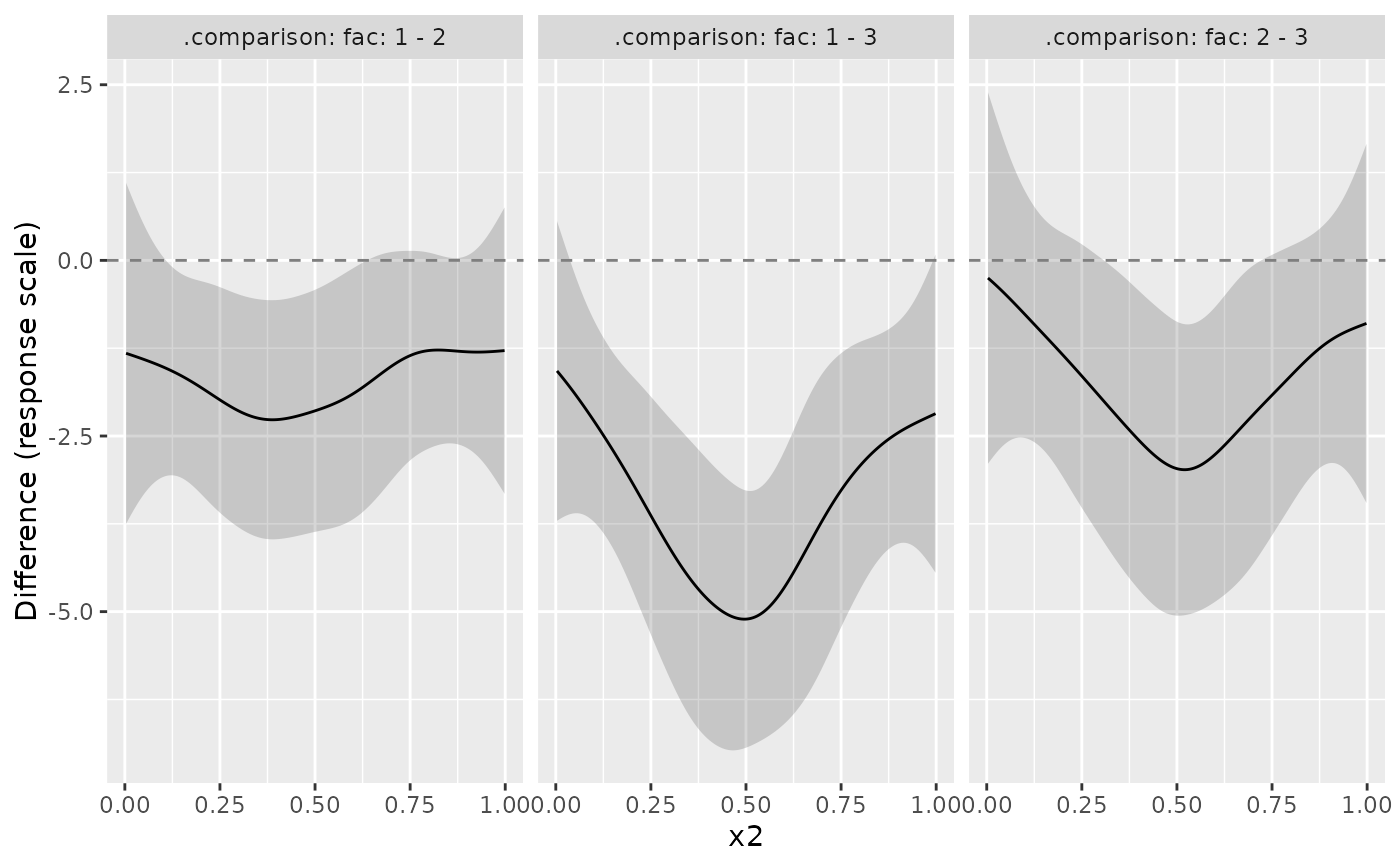
draw(cd)
 # Restrict comparisons and fix a further covariate
conditional_differences(m, by = "fac",
condition = list("x2", fac = c("1", "3"), x0 = 0.5))
#> # A tibble: 100 x 9
#> .contrast .level_1 .level_2 .diff .se .lower_ci .upper_ci x2 x0
#> <int> <fct> <fct> <dbl> <dbl> <dbl> <dbl> <dbl> <dbl>
#> 1 1 1 3 0.375 0.927 -1.44 2.19 0.00325 0.5
#> 2 1 1 3 0.000823 0.834 -1.63 1.63 0.0133 0.5
#> 3 1 1 3 -0.374 0.748 -1.84 1.09 0.0233 0.5
#> 4 1 1 3 -0.752 0.673 -2.07 0.567 0.0334 0.5
#> 5 1 1 3 -1.13 0.612 -2.33 0.0656 0.0434 0.5
#> 6 1 1 3 -1.52 0.566 -2.63 -0.413 0.0535 0.5
#> 7 1 1 3 -1.92 0.536 -2.97 -0.869 0.0635 0.5
#> 8 1 1 3 -2.33 0.518 -3.34 -1.31 0.0736 0.5
#> 9 1 1 3 -2.74 0.509 -3.74 -1.74 0.0836 0.5
#> 10 1 1 3 -3.16 0.505 -4.15 -2.17 0.0937 0.5
#> # i 90 more rows
# Pointwise posterior bands from shared coefficient draws
conditional_differences(m, by = "fac", condition = "x2",
uncertainty = "simulation", n_sim = 1000, seed = 42)
#> # A tibble: 300 x 9
#> .contrast .level_1 .level_2 .diff .se .lower_ci .upper_ci x2 x0
#> <int> <fct> <fct> <dbl> <dbl> <dbl> <dbl> <dbl> <dbl>
#> 1 1 1 2 2.76 0.878 1.05 4.51 0.00325 0.462
#> 2 1 1 2 2.80 0.830 1.15 4.45 0.0133 0.462
#> 3 1 1 2 2.85 0.784 1.29 4.42 0.0233 0.462
#> 4 1 1 2 2.89 0.741 1.43 4.34 0.0334 0.462
#> 5 1 1 2 2.94 0.699 1.55 4.32 0.0434 0.462
#> 6 1 1 2 2.98 0.660 1.67 4.25 0.0535 0.462
#> 7 1 1 2 3.03 0.625 1.81 4.23 0.0635 0.462
#> 8 1 1 2 3.07 0.592 1.93 4.19 0.0736 0.462
#> 9 1 1 2 3.11 0.562 2.01 4.19 0.0836 0.462
#> 10 1 1 2 3.16 0.536 2.10 4.20 0.0937 0.462
#> # i 290 more rows
# Link-scale simultaneous bands, separately for each comparison
conditional_differences(m, by = "fac", condition = "x2", scale = "link",
interval = "simultaneous", n_vals = 200, n_sim = 1000, seed = 42)
#> # A tibble: 600 x 10
#> .contrast .level_1 .level_2 .diff .se .lower_ci .upper_ci x2 x0
#> <int> <fct> <fct> <dbl> <dbl> <dbl> <dbl> <dbl> <dbl>
#> 1 1 1 2 2.76 0.859 0.338 5.18 0.00325 0.462
#> 2 1 1 2 2.78 0.836 0.424 5.14 0.00825 0.462
#> 3 1 1 2 2.80 0.814 0.509 5.10 0.0132 0.462
#> 4 1 1 2 2.83 0.792 0.593 5.06 0.0182 0.462
#> 5 1 1 2 2.85 0.770 0.675 5.02 0.0232 0.462
#> 6 1 1 2 2.87 0.749 0.756 4.98 0.0282 0.462
#> 7 1 1 2 2.89 0.729 0.836 4.95 0.0332 0.462
#> 8 1 1 2 2.91 0.709 0.913 4.92 0.0382 0.462
#> 9 1 1 2 2.94 0.690 0.989 4.88 0.0432 0.462
#> 10 1 1 2 2.96 0.672 1.06 4.85 0.0482 0.462
#> # i 590 more rows
#> # i 1 more variable: .crit <dbl>
# Nonlinear response differences: simultaneous coverage across all pairs
set.seed(42)
df$count <- rpois(nrow(df), exp(0.2 + sin(3 * df$x2) + as.integer(df$fac) / 3))
mp <- gam(count ~ fac + s(x2, by = fac), family = poisson(),
data = df, method = "REML")
conditional_differences(mp, by = "fac", condition = "x2", scale = "response",
uncertainty = "simulation", interval = "simultaneous",
simultaneous_scope = "all", n_vals = 200, n_sim = 1000, seed = 42) |>
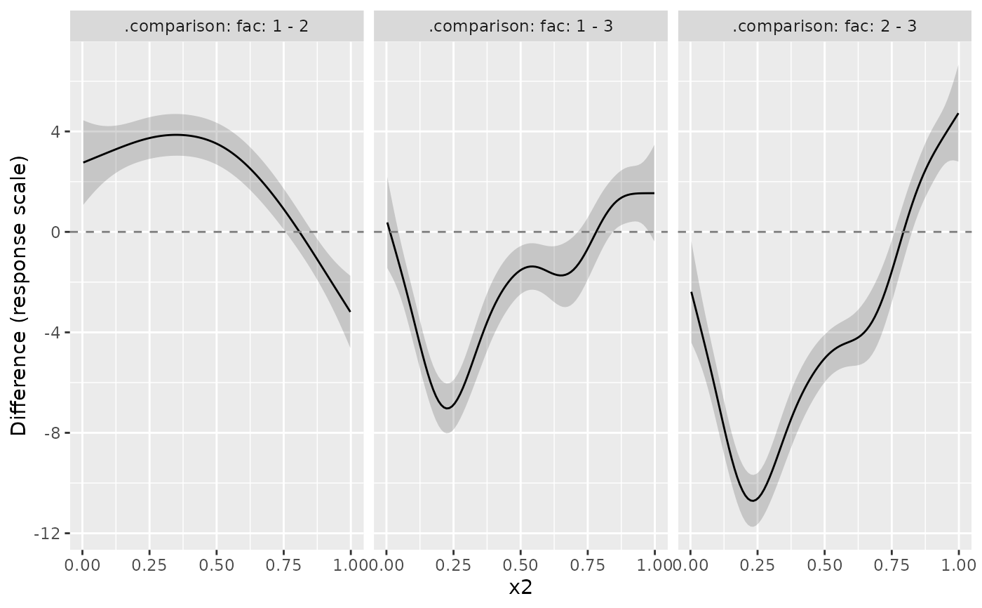
draw()
# Restrict comparisons and fix a further covariate
conditional_differences(m, by = "fac",
condition = list("x2", fac = c("1", "3"), x0 = 0.5))
#> # A tibble: 100 x 9
#> .contrast .level_1 .level_2 .diff .se .lower_ci .upper_ci x2 x0
#> <int> <fct> <fct> <dbl> <dbl> <dbl> <dbl> <dbl> <dbl>
#> 1 1 1 3 0.375 0.927 -1.44 2.19 0.00325 0.5
#> 2 1 1 3 0.000823 0.834 -1.63 1.63 0.0133 0.5
#> 3 1 1 3 -0.374 0.748 -1.84 1.09 0.0233 0.5
#> 4 1 1 3 -0.752 0.673 -2.07 0.567 0.0334 0.5
#> 5 1 1 3 -1.13 0.612 -2.33 0.0656 0.0434 0.5
#> 6 1 1 3 -1.52 0.566 -2.63 -0.413 0.0535 0.5
#> 7 1 1 3 -1.92 0.536 -2.97 -0.869 0.0635 0.5
#> 8 1 1 3 -2.33 0.518 -3.34 -1.31 0.0736 0.5
#> 9 1 1 3 -2.74 0.509 -3.74 -1.74 0.0836 0.5
#> 10 1 1 3 -3.16 0.505 -4.15 -2.17 0.0937 0.5
#> # i 90 more rows
# Pointwise posterior bands from shared coefficient draws
conditional_differences(m, by = "fac", condition = "x2",
uncertainty = "simulation", n_sim = 1000, seed = 42)
#> # A tibble: 300 x 9
#> .contrast .level_1 .level_2 .diff .se .lower_ci .upper_ci x2 x0
#> <int> <fct> <fct> <dbl> <dbl> <dbl> <dbl> <dbl> <dbl>
#> 1 1 1 2 2.76 0.878 1.05 4.51 0.00325 0.462
#> 2 1 1 2 2.80 0.830 1.15 4.45 0.0133 0.462
#> 3 1 1 2 2.85 0.784 1.29 4.42 0.0233 0.462
#> 4 1 1 2 2.89 0.741 1.43 4.34 0.0334 0.462
#> 5 1 1 2 2.94 0.699 1.55 4.32 0.0434 0.462
#> 6 1 1 2 2.98 0.660 1.67 4.25 0.0535 0.462
#> 7 1 1 2 3.03 0.625 1.81 4.23 0.0635 0.462
#> 8 1 1 2 3.07 0.592 1.93 4.19 0.0736 0.462
#> 9 1 1 2 3.11 0.562 2.01 4.19 0.0836 0.462
#> 10 1 1 2 3.16 0.536 2.10 4.20 0.0937 0.462
#> # i 290 more rows
# Link-scale simultaneous bands, separately for each comparison
conditional_differences(m, by = "fac", condition = "x2", scale = "link",
interval = "simultaneous", n_vals = 200, n_sim = 1000, seed = 42)
#> # A tibble: 600 x 10
#> .contrast .level_1 .level_2 .diff .se .lower_ci .upper_ci x2 x0
#> <int> <fct> <fct> <dbl> <dbl> <dbl> <dbl> <dbl> <dbl>
#> 1 1 1 2 2.76 0.859 0.338 5.18 0.00325 0.462
#> 2 1 1 2 2.78 0.836 0.424 5.14 0.00825 0.462
#> 3 1 1 2 2.80 0.814 0.509 5.10 0.0132 0.462
#> 4 1 1 2 2.83 0.792 0.593 5.06 0.0182 0.462
#> 5 1 1 2 2.85 0.770 0.675 5.02 0.0232 0.462
#> 6 1 1 2 2.87 0.749 0.756 4.98 0.0282 0.462
#> 7 1 1 2 2.89 0.729 0.836 4.95 0.0332 0.462
#> 8 1 1 2 2.91 0.709 0.913 4.92 0.0382 0.462
#> 9 1 1 2 2.94 0.690 0.989 4.88 0.0432 0.462
#> 10 1 1 2 2.96 0.672 1.06 4.85 0.0482 0.462
#> # i 590 more rows
#> # i 1 more variable: .crit <dbl>
# Nonlinear response differences: simultaneous coverage across all pairs
set.seed(42)
df$count <- rpois(nrow(df), exp(0.2 + sin(3 * df$x2) + as.integer(df$fac) / 3))
mp <- gam(count ~ fac + s(x2, by = fac), family = poisson(),
data = df, method = "REML")
conditional_differences(mp, by = "fac", condition = "x2", scale = "response",
uncertainty = "simulation", interval = "simultaneous",
simultaneous_scope = "all", n_vals = 200, n_sim = 1000, seed = 42) |>
draw()