Working with shape-constrained additive models • gratia

gratia supports the 24 univariate and 17 bivariate smooth constructors in scam 1.2-22, including cyclic margins, endpoint constraints, local constraints, by smooths and smooth interactions. Ordinary mgcv smooths fitted through scam() are also supported. The same fitted coefficient mapping is used for smooth estimates, bases, derivatives, predictions and sampled smooths.

library("mgcv")
library("scam")
library("gratia")

set.seed(46)
d <- data.frame(x = runif(200), z = runif(200))
d$y <- exp(d$x) + d$z + rnorm(nrow(d), sd = 0.15)
m <- scam(y ~ s(x, bs = "mpi", k = 8) + s(z, bs = "mpi", k = 8),
  data = d, not.exp = TRUE)
draw(m)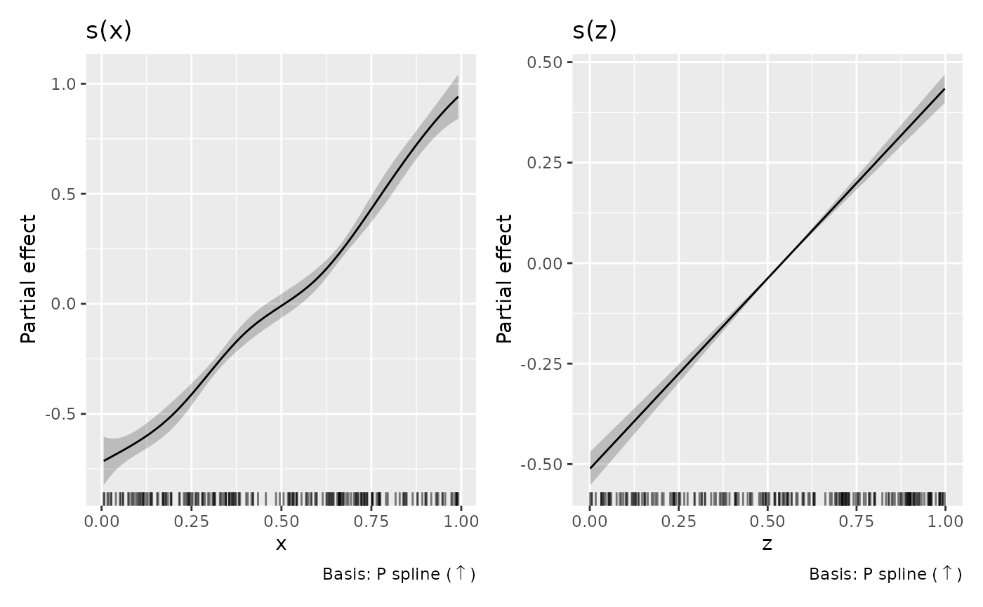

Fitted functions and native plots

Plot captions describe basis and shape separately. Increasing and decreasing constraints use arrows; tensor captions name the covariate for each constraint. Local constraints show their fitted change point. These captions are also available when drawing saved smooth_estimates(). The .type column and smooth_type() retain compact ASCII labels such as P spline (inc) and Tensor (inc, free).

By default, draw() retains the fitted function’s centring. Evaluating a smooth on a different grid therefore evaluates the same function. This agrees with scam’s univariate plots. Its bivariate plots instead subtract the mean of the evaluated surface. Use centre = "plot" to match that convention; both estimates and their covariance receive the same centring operation. assemble() accepts the same argument. Match grids and exclusion distances when comparing plots from the two packages.

b <- scam(y ~ s(x, z, bs = "tedmi", k = c(5, 5)), data = d,
  not.exp = TRUE)
draw(b, centre = "plot", n_2d = 40)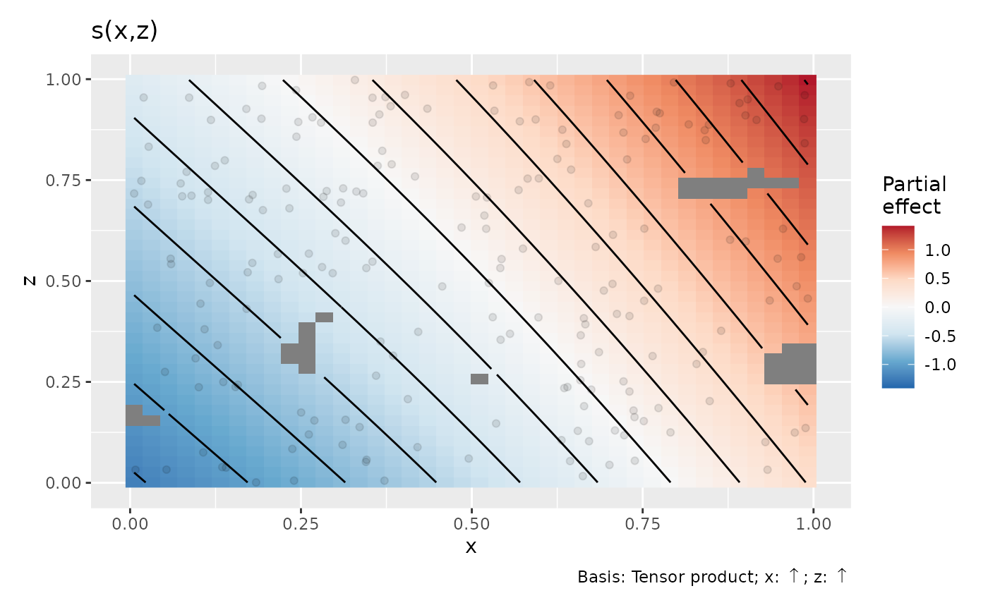

scam’s default univariate limits use two standard errors; gratia’s default 95% normal limits use qnorm(0.975). Some scam smooth classes also use a different coefficient gradient for the displayed function and its standard error. gratia computes uncertainty for the actual function it returns, using its coefficient gradient. This can produce different limits even when the fitted curves agree.

Conditional uncertainty and sampled functions

Pointwise intervals, simultaneous smooth bands, smooth derivatives and contrasts use scam’s covariance for the transformed coefficients (Vp.t, or Ve.t with frequentist = TRUE). These are local Gaussian or delta approximations, conditional on the fitted smoothing parameters. Including intercept uncertainty is controlled by overall_uncertainty.

e <- smooth_estimates(m, overall_uncertainty = FALSE)
e <- add_confint(e)
head(e)
#> # A tibble: 6 × 9
#>   .smooth .type         .by   .estimate    .se       x     z .lower_ci .upper_ci
#>   <chr>   <chr>         <chr>     <dbl>  <dbl>   <dbl> <dbl>     <dbl>     <dbl>
#> 1 s(x)    P spline (in… NA       -0.714 0.0561 0.00591    NA    -0.824    -0.604
#> 2 s(x)    P spline (in… NA       -0.705 0.0490 0.0159     NA    -0.801    -0.609
#> 3 s(x)    P spline (in… NA       -0.696 0.0431 0.0258     NA    -0.781    -0.612
#> 4 s(x)    P spline (in… NA       -0.687 0.0383 0.0358     NA    -0.762    -0.612
#> 5 s(x)    P spline (in… NA       -0.678 0.0346 0.0457     NA    -0.746    -0.611
#> 6 s(x)    P spline (in… NA       -0.669 0.0318 0.0557     NA    -0.732    -0.607
derivatives(m, select = "s(x)")
#> # A tibble: 100 × 9
#>    .smooth .by   .fs   .derivative   .se .crit .lower_ci .upper_ci       x
#>    <chr>   <chr> <chr>       <dbl> <dbl> <dbl>     <dbl>     <dbl>   <dbl>
#>  1 s(x)    NA    NA          0.901 0.963  1.96   -0.986       2.79 0.00591
#>  2 s(x)    NA    NA          0.895 0.865  1.96   -0.800       2.59 0.0159 
#>  3 s(x)    NA    NA          0.893 0.774  1.96   -0.625       2.41 0.0258 
#>  4 s(x)    NA    NA          0.895 0.692  1.96   -0.462       2.25 0.0358 
#>  5 s(x)    NA    NA          0.902 0.619  1.96   -0.311       2.11 0.0457 
#>  6 s(x)    NA    NA          0.914 0.553  1.96   -0.171       2.00 0.0557 
#>  7 s(x)    NA    NA          0.930 0.496  1.96   -0.0434      1.90 0.0657 
#>  8 s(x)    NA    NA          0.950 0.448  1.96    0.0730      1.83 0.0756 
#>  9 s(x)    NA    NA          0.975 0.406  1.96    0.179       1.77 0.0856 
#> 10 s(x)    NA    NA          1.01  0.372  1.96    0.276       1.73 0.0955 
#> # ℹ 90 more rows
confint(m, parm = "s(x)", type = "simultaneous", seed = 53)
#> # A tibble: 100 × 9
#>    .smooth .type        .by         x .estimate    .se .crit .lower_ci .upper_ci
#>    <chr>   <chr>        <chr>   <dbl>     <dbl>  <dbl> <dbl>     <dbl>     <dbl>
#>  1 s(x)    P spline (i… NA    0.00591    -0.714 0.0561  2.85    -0.874    -0.554
#>  2 s(x)    P spline (i… NA    0.0159     -0.705 0.0490  2.85    -0.845    -0.565
#>  3 s(x)    P spline (i… NA    0.0258     -0.696 0.0431  2.85    -0.819    -0.573
#>  4 s(x)    P spline (i… NA    0.0358     -0.687 0.0383  2.85    -0.796    -0.578
#>  5 s(x)    P spline (i… NA    0.0457     -0.678 0.0346  2.85    -0.777    -0.580
#>  6 s(x)    P spline (i… NA    0.0557     -0.669 0.0318  2.85    -0.760    -0.578
#>  7 s(x)    P spline (i… NA    0.0657     -0.660 0.0300  2.85    -0.745    -0.575
#>  8 s(x)    P spline (i… NA    0.0756     -0.651 0.0288  2.85    -0.733    -0.568
#>  9 s(x)    P spline (i… NA    0.0856     -0.641 0.0283  2.85    -0.722    -0.560
#> 10 s(x)    P spline (i… NA    0.0955     -0.631 0.0281  2.85    -0.712    -0.551
#> # ℹ 90 more rows

Coefficient sampling uses a different approximation: draw a Gaussian vector in the unrestricted fitting coordinates using Vp (or Ve), then apply the positivity transformation used in the fit. This preserves the fitted shape constraints. This is a Gaussian approximation in fitting coordinates, rather than an exact constrained posterior. Because the transformation is nonlinear, these samples need not have the mean or covariance used for analytic intervals. Individual analytic interval endpoints need not satisfy the shape constraint.

Fitted, smooth, derivative and response sampling functions project these same transformed coefficient draws. response_derivatives() also uses them with its default uncertainty = "simulation"; uncertainty = "delta" instead uses the local transformed-coefficient covariance.

draws <- gaussian_draws(m, n_draws = 100, seed = 54)
samples <- smooth_samples(m, n_draws = 5, seed = 55)
head(samples)
#> # A tibble: 6 × 9
#>   .smooth .term .type          .by    .row .draw .value       x     z
#>   <chr>   <chr> <chr>          <chr> <int> <int>  <dbl>   <dbl> <dbl>
#> 1 s(x)    s(x)  P spline (inc) NA        1     1 -1.00  0.00591    NA
#> 2 s(x)    s(x)  P spline (inc) NA        1     2 -0.853 0.00591    NA
#> 3 s(x)    s(x)  P spline (inc) NA        1     3 -0.749 0.00591    NA
#> 4 s(x)    s(x)  P spline (inc) NA        1     4 -0.922 0.00591    NA
#> 5 s(x)    s(x)  P spline (inc) NA        1     5 -0.898 0.00591    NA
#> 6 s(x)    s(x)  P spline (inc) NA        2     1 -0.985 0.0109     NA

method = "user" requires finite draws in the transformed coordinates, with columns in coef(m) order and nonnegative constrained coefficients. gaussian_draws(m, parametrized = FALSE) returns unrestricted draws for inspection; these cannot be supplied as transformed draws. A singular positive semidefinite covariance is supported. A materially indefinite covariance is rejected. When a very large unrestricted variance causes the exponential transformation to overflow, sampling reports an error; it does not truncate those draws. Finite transformed draws from an appropriate alternative sampler can still be supplied.

Other GAM operations

Supported methods include model summaries and term extraction, parametric effects, fitted and conditional predictions, smooth differences, analytic response derivatives, accumulated local effects, residual helpers, concurvity, penalties and response diagnostics. lp_matrix() and model.matrix() return a design whose columns match coef(m). Formula expressions retain their fitted prediction parameters, formula offsets are evaluated on new data, and training predictions also retain an offset argument used in fitting. Missing-row handling is shared across these methods.

Likelihood evaluation and LOO/WAIC use the supported independent-response family adapters, conditional on smoothing and other fitted family parameters. They use the same coefficient sampling approximation described above. variance_comp() reports response scale divided by smoothing parameters; these ratios describe penalties on unrestricted fitting parameters. They are not Gaussian variances of the transformed smooth coefficients, and their confidence limits are unavailable.

For Gaussian identity-link fits with AR1 dependence, response simulation uses the fitted correlation and AR.start series boundaries, including observation weights. It requires the fitting observations: a joint correlation structure for arbitrary new data is not defined. Other families with scam’s working AR1 correction do not automatically have a joint response simulator. Independent pointwise likelihood adapters reject correlated fits.

GCV and UBRE fits do not supply the smoothing-parameter covariance needed for unconditional = TRUE, unconditional EDF, or likelihood-based confidence limits for variance components. MH and INLA coefficient sampling are also unavailable. model_edf(type = "unconditional") follows the shared GAM convention: it warns and returns standard EDF when the correction is missing. Automatic interval_method = "shape" integration remains specific to supported scasm smooths; shape_intervals() can be used explicitly on supplied estimates and grids when its named shape restrictions apply.