Getting started with gratia • gratia

library("gratia")
#> Error in get(paste0(generic, ".", class), envir = get_method_env()) : 
#>   object 'type_sum.accel' not found
library("mgcv")
#> Loading required package: nlme
#> This is mgcv 1.9-1. For overview type 'help("mgcv-package")'.

gratia is a package to make working with generalized additive models (GAMs) in R easier, including producing plots of estimated smooths using the ggplot2 📦.

This introduction will cover some of the basic functionality of gratia to get you started. We’ll work with some classic simulated data often used to illustrate properties of GAMs

df <- data_sim("eg1", seed = 42)
df
#> # A tibble: 400 × 10
#>        y    x0     x1    x2    x3     f    f0    f1     f2    f3
#>    <dbl> <dbl>  <dbl> <dbl> <dbl> <dbl> <dbl> <dbl>  <dbl> <dbl>
#>  1  2.99 0.915 0.0227 0.909 0.402  1.62 0.529  1.05 0.0397     0
#>  2  4.70 0.937 0.513  0.900 0.432  3.25 0.393  2.79 0.0630     0
#>  3 13.9  0.286 0.631  0.192 0.664 13.5  1.57   3.53 8.41       0
#>  4  5.71 0.830 0.419  0.532 0.182  6.12 1.02   2.31 2.79       0
#>  5  7.63 0.642 0.879  0.522 0.838 10.4  1.80   5.80 2.76       0
#>  6  9.80 0.519 0.108  0.160 0.917 10.4  2.00   1.24 7.18       0
#>  7 10.4  0.737 0.980  0.520 0.798 11.3  1.47   7.10 2.75       0
#>  8 12.8  0.135 0.265  0.225 0.503 11.4  0.821  1.70 8.90       0
#>  9 13.8  0.657 0.0843 0.282 0.254 11.1  1.76   1.18 8.20       0
#> 10  7.51 0.705 0.386  0.504 0.667  6.50 1.60   2.16 2.74       0
#> # ℹ 390 more rows

and the following GAM

m <- gam(y ~ s(x0) + s(x1) + s(x2) + s(x3), data = df, method = "REML")
summary(m)
#> 
#> Family: gaussian 
#> Link function: identity 
#> 
#> Formula:
#> y ~ s(x0) + s(x1) + s(x2) + s(x3)
#> 
#> Parametric coefficients:
#>             Estimate Std. Error t value Pr(>|t|)    
#> (Intercept)   7.4951     0.1051   71.35   <2e-16 ***
#> ---
#> Signif. codes:  0 '***' 0.001 '**' 0.01 '*' 0.05 '.' 0.1 ' ' 1
#> 
#> Approximate significance of smooth terms:
#>         edf Ref.df      F  p-value    
#> s(x0) 3.425  4.244  8.828 8.78e-07 ***
#> s(x1) 3.221  4.003 67.501  < 2e-16 ***
#> s(x2) 7.905  8.685 67.766  < 2e-16 ***
#> s(x3) 1.885  2.359  2.642   0.0636 .  
#> ---
#> Signif. codes:  0 '***' 0.001 '**' 0.01 '*' 0.05 '.' 0.1 ' ' 1
#> 
#> R-sq.(adj) =  0.685   Deviance explained = 69.8%
#> -REML = 886.93  Scale est. = 4.4144    n = 400

Plotting

gratia provides the draw() function to produce plots using the ggplot2 📦. To plot the estimated smooths from the GAM we fitted above, use

draw(m)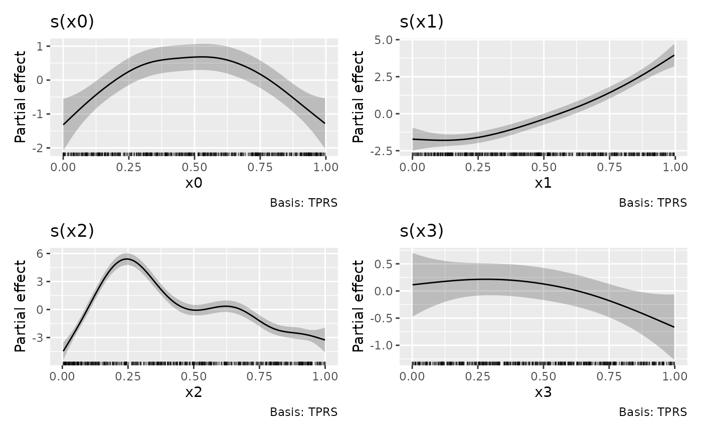

The plots produced are partial effect plots, which show the component contributions, on the link scale, of each model term to the linear predictor. The y axis on these plots is typically centred around 0 due to most smooths having a sum-to-zero identifiability constraint applied to them. This constraint is what allows the model to include multiple smooths and remain identifiable. These plots allow you to read off the contributions of each smooth to the fitted response (on the link scale); they show link-scale predictions of the response for each smooth, conditional upon all other terms in the model, including any parametric effects and the intercept, having zero contribution. In the parlance of the marginaleffects package (Arel-Bundock, Greifer, and Heiss Forthcoming), these plots show adjusted predictions, just where the adjustment includes setting the contribution of all other model terms to the predicted value to zero. For partial derivatives (what marginaleffects would call a marginal effect or slope), gratia provides derivatives().

The resulting plot is intended as reasonable overview of the estimated model, but it offers limited option to modify the resulting plot. If you want full control, you can obtain the data used to create the plot above with smooth_estimates()

sm <- smooth_estimates(m)
sm
#> # A tibble: 400 × 9
#>    .smooth .type .by   .estimate   .se       x0    x1    x2    x3
#>    <chr>   <chr> <chr>     <dbl> <dbl>    <dbl> <dbl> <dbl> <dbl>
#>  1 s(x0)   TPRS  NA       -1.32  0.390 0.000239    NA    NA    NA
#>  2 s(x0)   TPRS  NA       -1.24  0.365 0.0103      NA    NA    NA
#>  3 s(x0)   TPRS  NA       -1.17  0.340 0.0204      NA    NA    NA
#>  4 s(x0)   TPRS  NA       -1.09  0.318 0.0304      NA    NA    NA
#>  5 s(x0)   TPRS  NA       -1.02  0.297 0.0405      NA    NA    NA
#>  6 s(x0)   TPRS  NA       -0.947 0.279 0.0506      NA    NA    NA
#>  7 s(x0)   TPRS  NA       -0.875 0.263 0.0606      NA    NA    NA
#>  8 s(x0)   TPRS  NA       -0.803 0.249 0.0707      NA    NA    NA
#>  9 s(x0)   TPRS  NA       -0.732 0.237 0.0807      NA    NA    NA
#> 10 s(x0)   TPRS  NA       -0.662 0.228 0.0908      NA    NA    NA
#> # ℹ 390 more rows

which will evaluate all smooths at values that are evenly spaced over the range of the covariate(s). If you want to evaluate only selected smooths, you can specify which via the smooth argument. This takes the smooth labels which are the names of the smooths as they are known to mgcv. To list the labels for the smooths in use

smooths(m)
#> [1] "s(x0)" "s(x1)" "s(x2)" "s(x3)"

To evaluate only $f(x_2)$ use

sm <- smooth_estimates(m, smooth = "s(x2)")
#> Warning: The `smooth` argument of `smooth_estimates()` is deprecated as of gratia
#> 0.8.9.9.
#> ℹ Please use the `select` argument instead.
#> This warning is displayed once every 8 hours.
#> Call `lifecycle::last_lifecycle_warnings()` to see where this warning was
#> generated.
sm
#> # A tibble: 100 × 6
#>    .smooth .type .by   .estimate   .se      x2
#>    <chr>   <chr> <chr>     <dbl> <dbl>   <dbl>
#>  1 s(x2)   TPRS  NA      -4.47   0.476 0.00359
#>  2 s(x2)   TPRS  NA      -4.00   0.406 0.0136 
#>  3 s(x2)   TPRS  NA      -3.53   0.345 0.0237 
#>  4 s(x2)   TPRS  NA      -3.06   0.295 0.0338 
#>  5 s(x2)   TPRS  NA      -2.58   0.263 0.0438 
#>  6 s(x2)   TPRS  NA      -2.09   0.250 0.0539 
#>  7 s(x2)   TPRS  NA      -1.59   0.253 0.0639 
#>  8 s(x2)   TPRS  NA      -1.08   0.264 0.0740 
#>  9 s(x2)   TPRS  NA      -0.564  0.278 0.0841 
#> 10 s(x2)   TPRS  NA      -0.0364 0.289 0.0941 
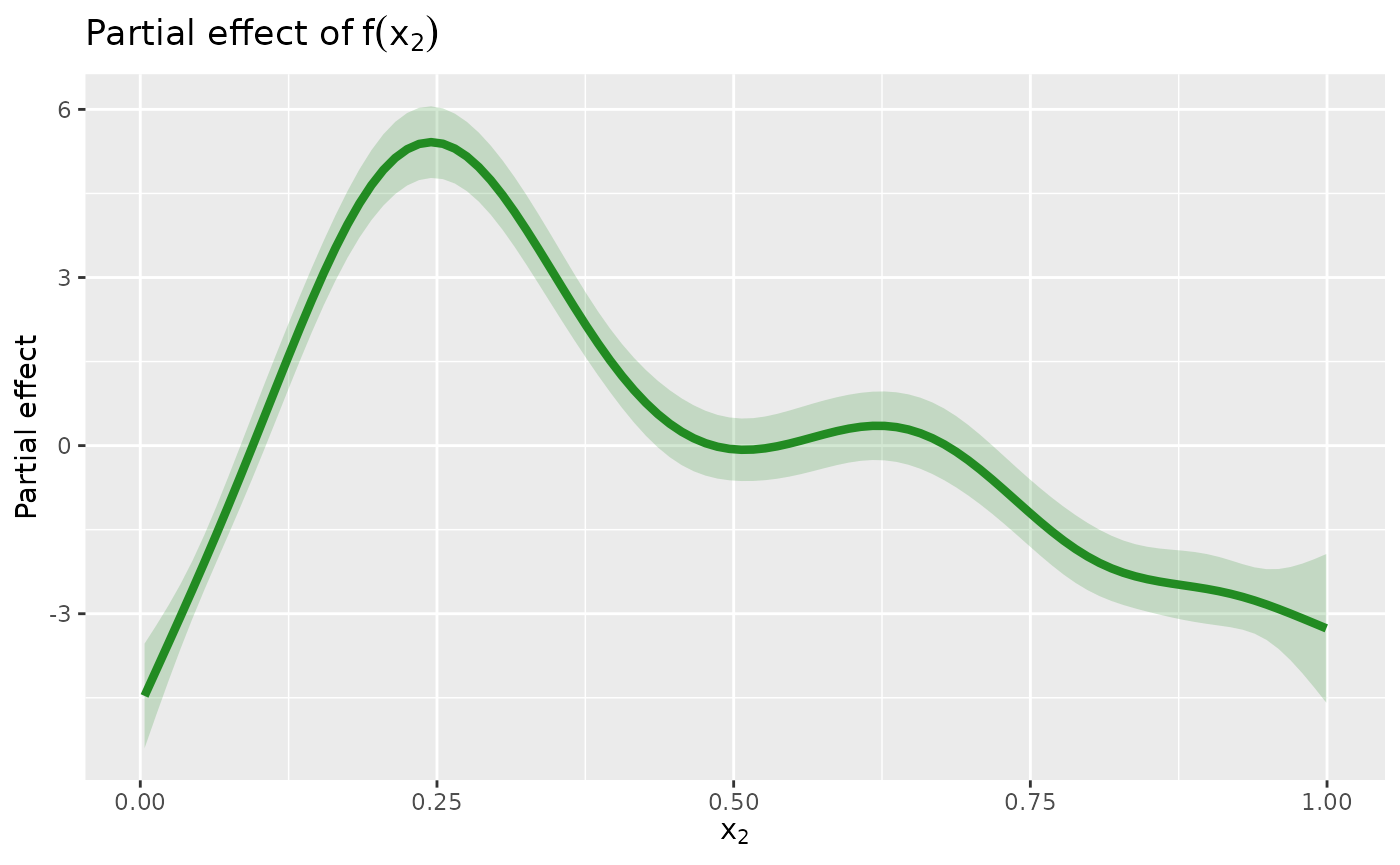
#> # ℹ 90 more rows

Then you can generate your own plot using the ggplot2 package, for example

library("ggplot2")
library("dplyr")
#> 
#> Attaching package: 'dplyr'
#> The following object is masked from 'package:nlme':
#> 
#>     collapse
#> The following objects are masked from 'package:stats':
#> 
#>     filter, lag
#> The following objects are masked from 'package:base':
#> 
#>     intersect, setdiff, setequal, union
sm |>
  add_confint() |>
  ggplot(aes(y = .estimate, x = x2)) +
  geom_ribbon(aes(ymin = .lower_ci, ymax = .upper_ci),
    alpha = 0.2, fill = "forestgreen"
  ) +
  geom_line(colour = "forestgreen", linewidth = 1.5) +
  labs(
    y = "Partial effect",
    title = expression("Partial effect of" ~ f(x[2])),
    x = expression(x[2])
  )

Model diagnostics

The appraise() function provides standard diagnostic plots for GAMs

appraise(m)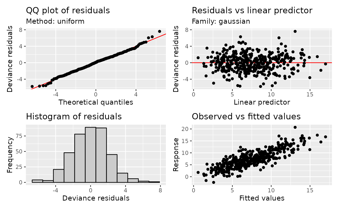

The plots produced are (from left-to-right, top-to-bottom),

a quantile-quantile (QQ) plot of deviance residuals,
a scatterplot of deviance residuals against the linear predictor,
a histogram of deviance residuals, and
a scatterplot of observed vs fitted values.

Adding partial residuals to the partial effect plots produced by draw() can also help diagnose problems with the model, such as oversmoothing

draw(m, residuals = TRUE)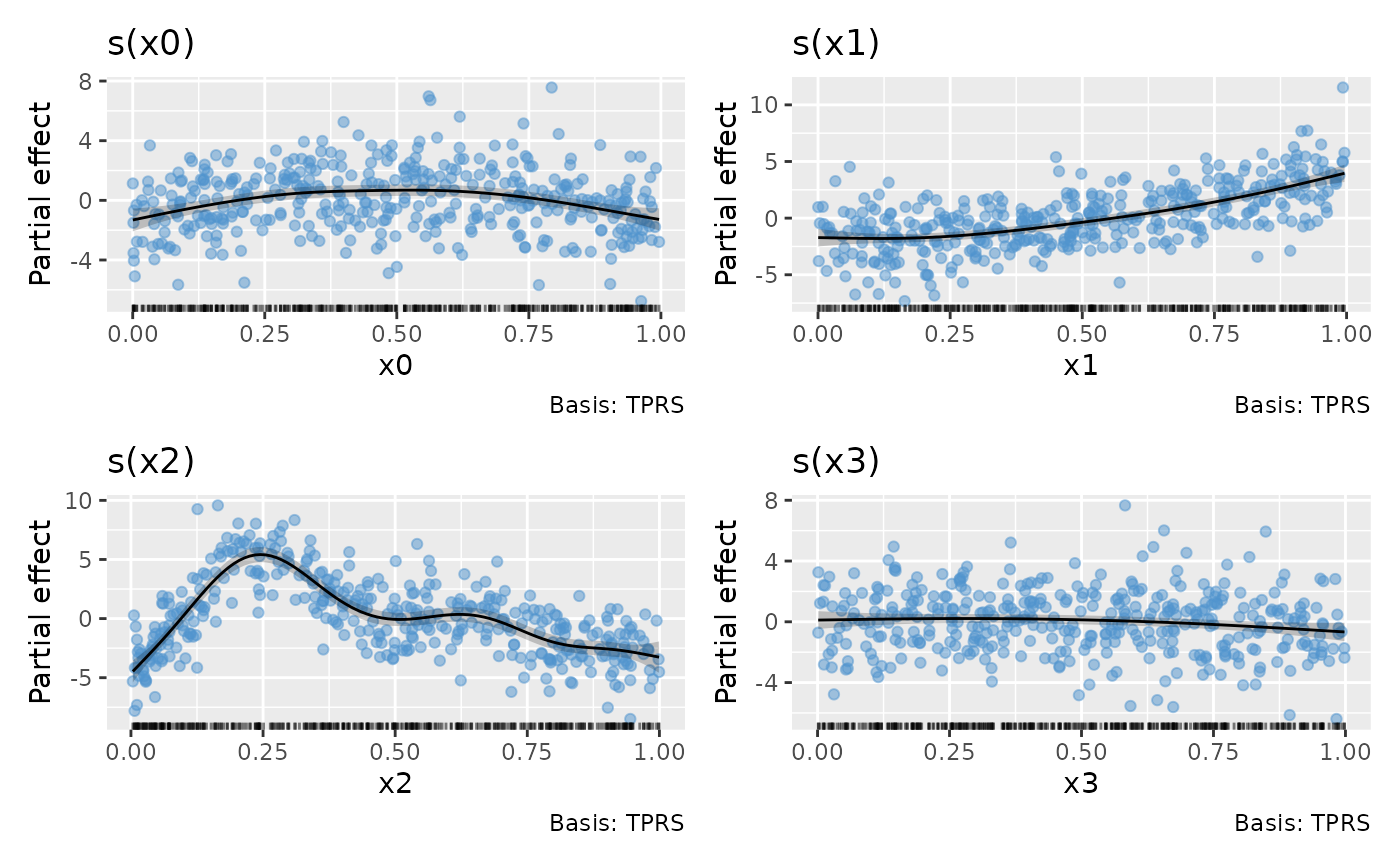

Want to learn more?

gratia is in very active development and an area of development that is currently lacking is documentation. To find out more about the package, look at the help pages for the package and look at the examples for more code to help you get going.

References

Arel-Bundock, Vincent, Noah Greifer, and Andrew Heiss. Forthcoming. “How to Interpret Statistical Models Using marginaleffects in R and Python.” Journal of Statistical Software, Forthcoming.