Evaluate smooths at covariate values — smooth

Evaluate a smooth at a grid of evenly spaced value over the range of the covariate associated with the smooth. Alternatively, a set of points at which the smooth should be evaluated can be supplied. smooth_estimates() is a new implementation of evaluate_smooth(), and replaces that function, which has been removed from the package.

Usage

smooth_estimates(object, ...)

# S3 method for class 'gam'
smooth_estimates(
  object,
  select = NULL,
  smooth = deprecated(),
  n = 100,
  n_2d = 50,
  n_3d = 16,
  n_4d = 4,
  data = NULL,
  unconditional = FALSE,
  frequentist = FALSE,
  overall_uncertainty = TRUE,
  dist = NULL,
  unnest = TRUE,
  partial_match = FALSE,
  clip = FALSE,
  envir = NULL,
  back_transform = FALSE,
  interval = NULL,
  ci_level = 0.95,
  n_sim = 10000,
  n_cores = 1,
  seed = NULL,
  interval_method = c("auto", "gaussian", "bootstrap", "shape"),
  shape_source = c("gaussian", "bootstrap"),
  ...,
  variables = NULL,
  simultaneous_method = c("simulation", "tube"),
  simultaneous_domain = NULL,
  tube_control = list()
)

# S3 method for class 'gamlss'
smooth_estimates(
  object,
  select = NULL,
  smooth = deprecated(),
  ...,
  partial_match = FALSE
)

Arguments

object: a fitted model, including objects of class "gam", "gamm" or models fitted by GJRM::gamlss().
...: arguments passed to other methods.
select: character, numeric or logical; smooths to evaluate, using labels from smooths() or indices in fitted smooth order. The default (NULL) evaluates all smooths.
smooth: Use select instead.
n: numeric; the number of points over the range of the covariate at which to evaluate a univariate smooth.
n_2d: numeric; the number of points along each of the first two axes of a smooth surface, including surface panels of higher-dimensional smooths. The default is 50 in plotting and plot-preparation functions. If NULL, use n instead. Ignored when evaluation data are supplied. Factor levels are retained, and curves with only one continuous covariate use n.
n_3d, n_4d: numeric; the number of points along the third axis of a 3D smooth (n_3d, default 16), or each axis after the first two for smooths of dimension four or higher (n_4d, default 4). If NULL, use n for those axes. For factor conditioning dimensions, retain at most that many levels, taking the first in fitted order. The first two surface axes use n_2d. Supplied data are unchanged.
data: a data frame of covariate values at which to evaluate the smooth.
unconditional: logical; if TRUE (and only if frequentist == FALSE) then the bayesian smoothing parameter uncertainty-corrected covariance matrix is returned, if available. Whether it is available depends on which smoothness selection method was used to fit the model.
frequentist: logical; if FALSE, the default, the bayesian covariance matrix is returned, otherwise the frequentist covariance matrix.
overall_uncertainty: logical; should the uncertainty in the model constant term be included in the standard error of the evaluate values of the smooth?
dist: numeric; if greater than 0, this is used to determine when a location is too far from data to be plotted when plotting 2-D smooths. The data are scaled into the unit square before deciding what to exclude, and dist is a distance within the unit square. See mgcv::exclude.too.far() for further details.
unnest: logical; unnest the smooth objects?
partial_match: logical; in the case of character select, should select match partially against smooths? If partial_match = TRUE, select must only be a single string, a character vector of length 1.
clip: logical; should evaluation points be clipped to the boundary of a soap film smooth? The default is FALSE, which will return NA for any point that is deemed to lie outside the boundary of the soap film.
envir: an optional environment supplying functions and constants used in model expressions. The available model formula environment is used when NULL. Covariate observations should be supplied in data.
back_transform: logical; generate automatic grids on the original covariate scale? The default, FALSE, preserves evenly spaced model-scale grids (e.g. in log(x)). With TRUE, recover raw fitting covariates and generate grids on their original scale, then evaluate the model expressions forwards. Each axis must depend on one distinct original model covariate. Functions such as foo(x) require no inverse. Fitted prediction parameters are retained where provided by the model, including for scale(x). When data are supplied, use those rows without generating a grid; TRUE requires raw coordinates for each axis. Returned model-coordinate columns keep their usual names and raw coordinates are retained in auxiliary .gratia_raw_* columns. Draw these estimates with draw(object, back_transform = TRUE) to display the raw coordinates. Estimates containing only transformed coordinates give an informative error if drawn on the original scale. This option does not change effect values or their intervals at the chosen evaluation points.
interval: character or NULL; NULL (the default) returns estimates and standard errors only. "confidence" adds pointwise intervals and "simultaneous" adds a band covering, by default, the finite evaluation grid of each fitted smooth. "credible" is an alias for "confidence"; the default Bayesian covariance gives approximate Bayesian credible intervals.
ci_level: numeric; interval coverage, strictly between zero and one.
n_sim, n_cores: positive integers; coefficient draws and simulation cores for simultaneous bands. Parallel simulation requires OpenMP support.
seed: integer or NULL; an explicit simulation seed preserves the caller's RNG state. Shared coefficient draws make results independent of selected smooth order and parallel evaluation scheduling.
interval_method: character; "auto" uses stored scasm bootstrap draws for pointwise intervals when available, and Gaussian intervals otherwise. Use "gaussian" to request covariance-based limits or "bootstrap" to require stored draws. Simultaneous bootstrap bands are not supported. "shape" applies shape_intervals() to supported scasm smooth components, using the initial limits chosen by shape_source.
shape_source: character; initial uncertainty for interval_method = "shape": "gaussian" (the default) or stored "bootstrap" pointwise limits. Bootstrap sources require frequentist = FALSE and unconditional = FALSE because the stored draws hold smoothing fixed.
variables: Character vector giving every covariate of the selected smooths exactly once, in plotting order: x, y, then the conditioning covariate for 3D smooths, or facet rows and columns for 4D smooths. When supplied, selected smooths must use the same covariates. Use fitted coordinate names, such as "log(x)" for a transformed covariate. The default, NULL, favours a two-variable tensor margin for x and y, otherwise retaining fitted order. Grid resolution follows this order. Supplied data are evaluated unchanged. Drawing saved estimates can change the order but uses only points already evaluated; evaluate again to change grid resolution or conditioning values. Continuous covariates must precede factors. Spherical smooths retain their latitude/longitude convention and do not support reordering.
simultaneous_method: character; calibration for simultaneous bands. The default, "simulation", uses coefficient draws on the evaluation grid. "tube" uses a conservative Gaussian threshold-crossing bound over a continuous interval for supported one-dimensional cubic splines. See simultaneous_bands.
simultaneous_domain: numeric pair of increasing finite endpoints, or a named list of such pairs keyed by spline coordinate. For tube bands, NULL uses the range of returned evaluation coordinates, including gaps. All returned points must lie inside the interval and the interval must lie inside the fitted spline support. Requires tube calibration.
tube_control: named list controlling numerical tube calibration: rel_tol (default 1e-6), abs_tol (1e-8), subdivisions (1000L), and root_tol (1e-8). Requires tube calibration. Simulation controls n_sim, n_cores (or ncores), and seed are ignored by tube calibration.

Value

A data frame (tibble), which is of class "smooth_estimates". Its plot_variables attribute is a list of resolved covariate orders, named by smooth label, used when drawing the saved estimates.

Details

For GJRM::gamlss() models, smooths are evaluated in equation and smooth order using the final fitted GJRM coefficients and covariance matrices. Selection uses the model-wide labels returned by smooths(), including suffixes such as s.1(x) for repeated labels. Equations without smooths are skipped; a model without any smooths gives an error. All grid, data, environment, coordinate transformation and interval controls are passed to the GAM method for each selected equation. frequentist = TRUE uses the final GJRM frequentist covariance. A smoothing-parameter uncertainty correction is unavailable: unconditional = TRUE warns and uses the uncorrected final covariance, as for GAMs without that correction.

For distributional and glmmTMB models with multiple linear predictors, an optional .model column identifies the model part or parameter associated with each smooth. This display metadata is retained in nested output and subsets, allowing draw() to reproduce model subtitles from saved estimates. Smooth labels and selection remain unchanged.

When distinct fitted terms share both their smooth label and type (for example, tensor products of soap-film components), .smooth_id contains their fitted smooth indices. This preserves their identity in saved estimates and plots without changing the labels supplied by mgcv.

By default, simultaneous coverage is per fitted smooth over its valid evaluation points, including all its slices and factor levels. Separate factor-by smooths remain separate coverage sets when grouped in one plot. This finite-grid band does not claim joint coverage across selected smooths or the full fitted model. Increasing grid resolution improves the approximation to whole-curve coverage. For supported univariate cubic splines, simultaneous_method = "tube" instead calibrates over a continuous interval; see simultaneous_bands. overall_uncertainty and covariance options apply to both interval types. SCAM smooth estimates retain the fitted centring and coefficient transformation when evaluation points are changed. Pointwise intervals use the covariance of the constrained coefficients. With overall_uncertainty = TRUE, their standard errors also include intercept uncertainty and its covariance with the smooth; estimates remain centred. Models without an intercept use smooth-only uncertainty for either setting. Native scasm fits use component-only uncertainty by default. Explicitly requesting overall_uncertainty = TRUE warns once if selected smooths lack the centring information needed to add mean uncertainty. Ordinary GAM defaults are unchanged.

Bootstrap pointwise limits follow mgcv's percentiles and its svar.only correction for smoothing bias. The correction can move limits beyond the fitted shape constraints. Estimates and covariance-based standard errors are unchanged; .crit is NA for asymmetric bootstrap limits. No new replicates are generated. Simultaneous intervals use Gaussian draws and warn if automatic selection leaves stored bootstrap draws unused.

The interval_info attribute records the interval source and correction. The shape_constraints attribute identifies requests and retained inequalities for each fitted smooth and tensor margin. Captions use plotmath arrows for increasing and decreasing constraints while .type and smooth_type() keep their existing basis names. Unsupported tensor requests produce a warning and are labelled as not retained.

SCAM captions describe the basis and its constraints separately from the compact .type values. Increasing and decreasing constraints use plotmath arrows. Tensor captions name each covariate and its constraint; local constraints include the fitted change point. The scam_smooth_info attribute preserves these descriptions when plotting saved estimates.

Shape enforcement is explicit and leaves the existing interval defaults unchanged. It preserves containment of a shape-restricted target whenever the entire initial band contains that target on the evaluation grid. This does not establish nominal coverage of the initial band, or preserve marginal coverage of transformed pointwise limits. The default Gaussian source uses approximate Bayesian covariance and does not construct a constrained posterior. Standard errors describe the initial calculation; .crit is NA after shape enforcement. Metadata records the initial source, correction, named shapes, model coordinates and whole-grid guarantee.

Every selected term must have retained named scasm restrictions. Supported combinations are positivity, monotonicity in any directions and curvature in at most one direction. Tensor smooths require te(..., np = FALSE) with univariate B-spline margins ("sc" or "bs"). Normal reparameterisation and other complementary bases can invalidate the named surface shape even when coefficient inequalities were retained. Curvature additionally requires equally spaced fitted knots to rounding precision and degree at least two. Irregular evaluation coordinates are supported. Complete product grids, finite endpoints and evaluation inside the fitted B-spline domains are required; use dist = 0 for tensors. Numeric by variables are unsupported; factor-by components and separate linear predictors are treated separately. Function-valued bases are required; derivative bases are unsupported. General pc inequalities can replace the named coefficient restrictions while leaving their original xt request in the fitted object. These replacements are labelled as general constraints and rejected for automatic shape intervals. Point equalities that retain the named inequalities are supported.

Shape intervals use component-only uncertainty: explicit overall_uncertainty = TRUE, effect shifts and effect transformations are rejected. Coordinate transformations used in the model remain supported; their named shapes concern model coordinates. The transformed endpoints need not belong to the fitted spline space or obey centring equalities. See shape_confidence_set() for explicit coefficient restrictions and the shape-constrained intervals article for examples.

Smoothing-parameter uncertainty is not currently supported for SCAM models; use unconditional = FALSE.

For explicit data, missing covariates needed by a smooth produce NA estimates and standard errors at those positions. Missing values in variables unrelated to that smooth do not discard its otherwise evaluable rows.

Raw data may contain x for a smooth such as s(log(x)); gratia evaluates the expression before constructing the prediction matrix. An evaluated column named "log(x)" can be supplied instead. When both are supplied, the raw inputs take precedence, except for stored model frames and grids prepared by gratia. Automatic grids are evenly spaced in the smooth coordinate (log(x)), and returned coordinate columns retain that name.

Stored evaluated columns allow automatic plotting even when a local function used to fit the model is no longer available. Evaluating that function at new raw data requires envir; training values are never substituted for new observations. Arbitrary transformations are not inverted to recover raw data. The coordinate_info attribute identifies retained raw coordinate columns. draw() uses them for back_transform = TRUE; the usual coordinate columns remain on the model scale. Automatic raw grids require recoverable fitting rows and matching functions and constants. Supplied raw data instead define the prediction rows directly. Typical covariate values added to evaluated grids by include_all = TRUE are not raw axis coordinates. Numeric by multipliers are set to one on automatic grids, even when their name also identifies a raw axis; supplied prediction rows retain their actual multipliers. Soap-film boundary rows retain model coordinates only. If a boundary axis is transformed, draw the estimates with back_transform = FALSE; raw-scale drawing gives an error rather than dropping the boundary.

Examples

load_mgcv()
dat <- data_sim("eg1", n = 400, dist = "normal", scale = 2, seed = 2)
m1 <- gam(y ~ s(x0) + s(x1) + s(x2) + s(x3), data = dat, method = "REML")

## evaluate all smooths
smooth_estimates(m1)
#> # A tibble: 400 x 9
#>    .smooth .type .by   .estimate      .se         x0    x1    x2    x3
#>    <chr>   <chr> <chr>     <dbl>    <dbl>      <dbl> <dbl> <dbl> <dbl>
#>  1 s(x0)   TPRS  NA    -0.966542 0.316118 0.00710904    NA    NA    NA
#>  2 s(x0)   TPRS  NA    -0.925391 0.297170 0.0171157     NA    NA    NA
#>  3 s(x0)   TPRS  NA    -0.884233 0.279256 0.0271224     NA    NA    NA
#>  4 s(x0)   TPRS  NA    -0.843050 0.262594 0.0371291     NA    NA    NA
#>  5 s(x0)   TPRS  NA    -0.801824 0.247376 0.0471358     NA    NA    NA
#>  6 s(x0)   TPRS  NA    -0.760536 0.233728 0.0571425     NA    NA    NA
#>  7 s(x0)   TPRS  NA    -0.719175 0.221701 0.0671492     NA    NA    NA
#>  8 s(x0)   TPRS  NA    -0.677736 0.211261 0.0771559     NA    NA    NA
#>  9 s(x0)   TPRS  NA    -0.636220 0.202303 0.0871626     NA    NA    NA
#> 10 s(x0)   TPRS  NA    -0.594641 0.194685 0.0971693     NA    NA    NA
#> # i 390 more rows

## or selected smooths
smooth_estimates(m1, select = c("s(x0)", "s(x1)"))
#> # A tibble: 200 x 7
#>    .smooth .type .by   .estimate      .se         x0    x1
#>    <chr>   <chr> <chr>     <dbl>    <dbl>      <dbl> <dbl>
#>  1 s(x0)   TPRS  NA    -0.966542 0.316118 0.00710904    NA
#>  2 s(x0)   TPRS  NA    -0.925391 0.297170 0.0171157     NA
#>  3 s(x0)   TPRS  NA    -0.884233 0.279256 0.0271224     NA
#>  4 s(x0)   TPRS  NA    -0.843050 0.262594 0.0371291     NA
#>  5 s(x0)   TPRS  NA    -0.801824 0.247376 0.0471358     NA
#>  6 s(x0)   TPRS  NA    -0.760536 0.233728 0.0571425     NA
#>  7 s(x0)   TPRS  NA    -0.719175 0.221701 0.0671492     NA
#>  8 s(x0)   TPRS  NA    -0.677736 0.211261 0.0771559     NA
#>  9 s(x0)   TPRS  NA    -0.636220 0.202303 0.0871626     NA
#> 10 s(x0)   TPRS  NA    -0.594641 0.194685 0.0971693     NA
#> # i 190 more rows

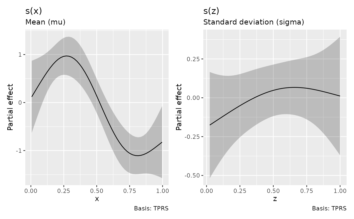
# Direct evaluation of a GJRM distributional model
if (requireNamespace("GJRM", quietly = TRUE)) {
  set.seed(82)
  d <- data.frame(x = runif(100), z = runif(100))
  d$y <- sin(6 * d$x) + rnorm(100, sd = exp(0.3 * d$z))
  m <- GJRM::gamlss(list(y ~ s(x, k = 4), ~ s(z, k = 4)), data = d)
  estimates <- smooth_estimates(m, n = 50)
  draw(estimates)
}


# parallel processing of smooths
if (requireNamespace("mirai") && requireNamespace("carrier")) {
  library("mirai")
  daemons(2)                          # only low for CRAN requirements
  smooth_estimates(m1)
}
#> # A tibble: 400 x 9
#>    .smooth .type .by   .estimate      .se         x0    x1    x2    x3
#>    <chr>   <chr> <chr>     <dbl>    <dbl>      <dbl> <dbl> <dbl> <dbl>
#>  1 s(x0)   TPRS  NA    -0.966542 0.316118 0.00710904    NA    NA    NA
#>  2 s(x0)   TPRS  NA    -0.925391 0.297170 0.0171157     NA    NA    NA
#>  3 s(x0)   TPRS  NA    -0.884233 0.279256 0.0271224     NA    NA    NA
#>  4 s(x0)   TPRS  NA    -0.843050 0.262594 0.0371291     NA    NA    NA
#>  5 s(x0)   TPRS  NA    -0.801824 0.247376 0.0471358     NA    NA    NA
#>  6 s(x0)   TPRS  NA    -0.760536 0.233728 0.0571425     NA    NA    NA
#>  7 s(x0)   TPRS  NA    -0.719175 0.221701 0.0671492     NA    NA    NA
#>  8 s(x0)   TPRS  NA    -0.677736 0.211261 0.0771559     NA    NA    NA
#>  9 s(x0)   TPRS  NA    -0.636220 0.202303 0.0871626     NA    NA    NA
#> 10 s(x0)   TPRS  NA    -0.594641 0.194685 0.0971693     NA    NA    NA
#> # i 390 more rows