Variance components in GAMs • gratia

This example uses variance_comp() to compare penalty variances with variances of fitted terms.

We simulate 360 observations in 12 groups of 30. The covariate z is a noisy version of x, so the two are positively correlated. We generate w independently for the nonlinear effect.

library("gratia")
load_mgcv()

set.seed(2026)
dat <- data.frame(x = runif(360, -1, 1), w = runif(360),
  group = factor(rep(seq_len(12), each = 30)))
dat$z <- 0.8 * dat$x + rnorm(360, sd = 0.2)

The response combines positive linear effects of x and z, a sine wave in w, differences between groups and Gaussian noise. Every observation in a group shares the same random intercept. Because the two linear effects tend to increase together, their covariance will contribute to the total variance.

group_effect <- rnorm(12, sd = 0.6)
dat$y <- 2 * dat$x + 1.5 * dat$z + sin(2 * pi * dat$w) +
  group_effect[dat$group] + rnorm(360, sd = 0.4)

We fit linear terms for x and z, a smooth for w and a random intercept for group. This gives us both unpenalised terms and terms with penalties to compare:

model <- gam(y ~ x + z + s(w, k = 8) + s(group, bs = "re"),
  data = dat, method = "REML")

Two kinds of variance

We first extract the penalty variances, which describe shrinkage of the penalised coefficients. The .lower_ci and .upper_ci columns give interval limits for standard deviations:

vc_penalty <- variance_comp(model, type = "penalty")
vc_penalty
#> # A tibble: 3 × 5
#>   .component .variance .std_dev .lower_ci .upper_ci
#>   <chr>          <dbl>    <dbl>     <dbl>     <dbl>
#> 1 s(w)         139.      11.8       6.51     21.3  
#> 2 s(group)       0.293    0.542     0.354     0.829
#> 3 scale          0.157    0.397     0.368     0.428

Penalty variances are \phi / \lambda_j: the model scale divided by the smoothing parameter. By default, the calculation undoes the rescaling that mgcv applies to penalties during fitting. Larger variances mean less shrinkage of the coefficients affected by that penalty. A smooth can have several penalties, each with its own row. Unpenalised terms such as x and z are omitted. For this Gaussian model, scale is the estimated residual variance.

With type = "terms", we instead measure how much each term’s fitted values vary across the observations used to fit the model. We use 1,000 coefficient draws for intervals and set a seed to make them reproducible:

vc_terms <- variance_comp(model, type = "terms", n_draws = 1000, seed = 42)
vc_terms
#> # A tibble: 5 × 8
#>   .component .variance .std_dev .lower_ci .upper_ci .proportion
#>   <chr>          <dbl>    <dbl>     <dbl>     <dbl>       <dbl>
#> 1 x              1.33     1.15      1.05      1.25       0.527 
#> 2 z              0.497    0.705     0.602     0.810      0.312 
#> 3 s(w)           0.497    0.705     0.665     0.747      0.115 
#> 4 s(group)       0.265    0.515     0.477     0.557      0.0466
#> 5 total          3.83     1.96      1.91      2.00       1     
#> # ℹ 2 more variables: .proportion_lower_ci <dbl>, .proportion_upper_ci <dbl>

These are sample variances on the linear predictor scale, with each observation counted equally. The output includes parametric terms and one row for each smooth, regardless of how many penalties it has. It excludes intercepts, offsets and residual variation.

Totals and proportions

The variance of the sum depends on both the term variances and their covariances. Let f_j be term j’s fitted values, F = \sum_j f_j their sum, and C their covariance matrix. Then

\operatorname{Var}(F) = \sum_j C_{jj} + 2\sum_{j<k} C_{jk}.

We retrieve the covariance matrix stored in the result to compare the sum of term variances with the total, which includes covariance:

C <- attr(vc_terms, "covariance")
c(sum_of_term_variances = sum(diag(C)),
  total_including_covariance = sum(C))
#>      sum_of_term_variances total_including_covariance 
#>                   2.588591                   3.829474

To divide the total among terms, we split each covariance contribution, 2C_{jk}, equally between the two terms. Each term’s proportion is then p_j = \operatorname{Cov}(f_j, F) / \operatorname{Var}(F). The individual terms’ proportions sum to one. We check this using include_total = FALSE to omit the total row and n_draws = 0 to skip interval calculations:

vc_no_total <- variance_comp(model, type = "terms", include_total = FALSE,
  n_draws = 0)
sum(vc_no_total$.proportion)
#> [1] 1

Penalty intervals use uncertainty in the estimated smoothing parameters and model scale. For term intervals, we draw all coefficients together from their approximate Gaussian posterior distribution. We recompute fitted values, variances and proportions for each draw, preserving dependence between terms. By default, the smoothing parameters stay fixed at their estimates. unconditional = TRUE adjusts for their uncertainty when that adjustment is available for the fitted model. The proportions from each draw are in attr(vc_terms, "proportion_draws")$total. Interval limits summarise each term separately and need not sum to one.

Plotting

We plot variances, including the total, alongside proportions for the individual terms. Both plots show intervals, with terms on the x-axis:

patchwork::wrap_plots(
  draw(vc_terms),
  draw(vc_terms, type = "proportion", include_total = FALSE),
  ncol = 2
)

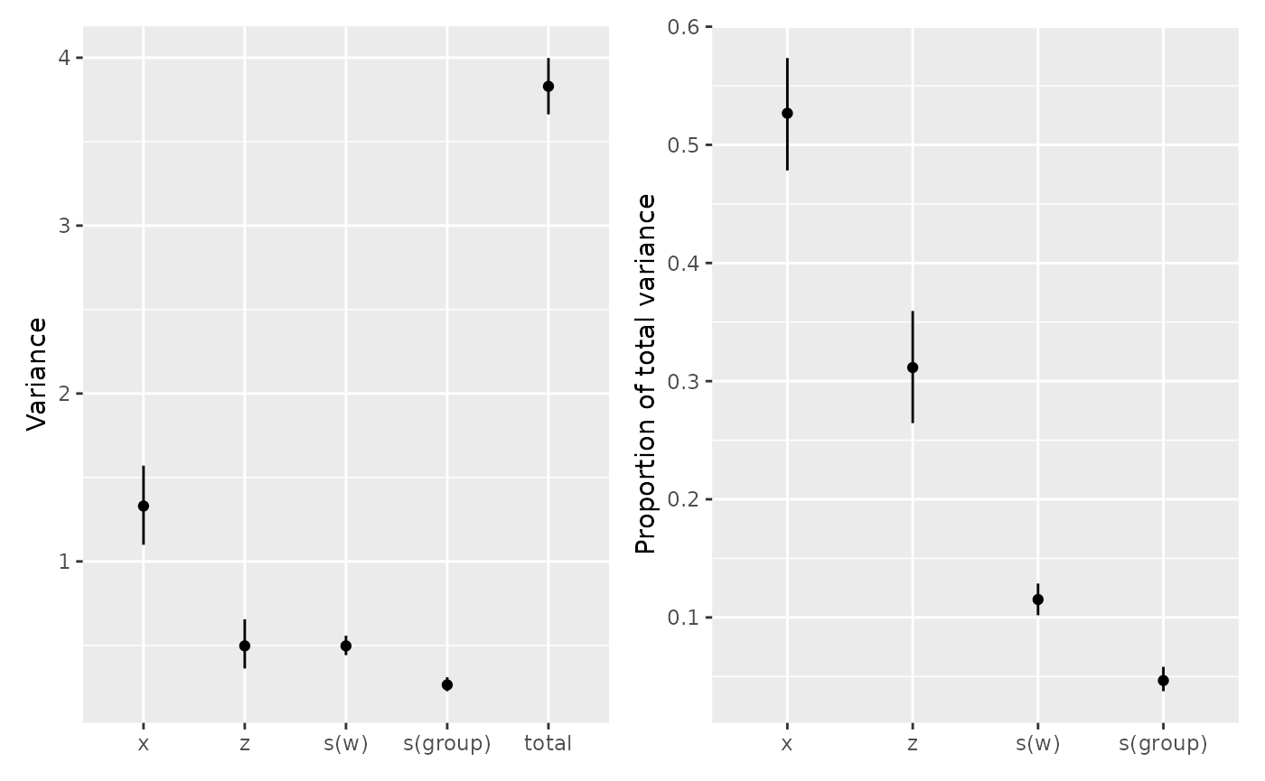
Use draw(vc_penalty) for penalty variances or draw(vc_terms, type = "std_dev") for term standard deviations. draw() uses the stored intervals, squaring standard deviation limits when plotting variances. Use n_dodge = 2 to stagger term labels, angle = 45 to rotate them, or flip = TRUE to put terms on the y-axis.

Negative proportions

To show how a proportion can be negative, we reuse the correlated x and z but give their effects opposite signs. The new response combines 2 * x - z with Gaussian noise of standard deviation 0.1, so the two effects partly cancel each other:

set.seed(208)
dat$contrast <- 2 * dat$x - dat$z + rnorm(nrow(dat), sd = 0.1)

We fit both linear terms and plot their proportions with intervals, omitting the total row:

opposing <- gam(contrast ~ x + z, data = dat, method = "REML")
vc_opposing <- variance_comp(opposing, type = "terms", n_draws = 1000, seed = 43)
draw(vc_opposing, type = "proportion", include_total = FALSE)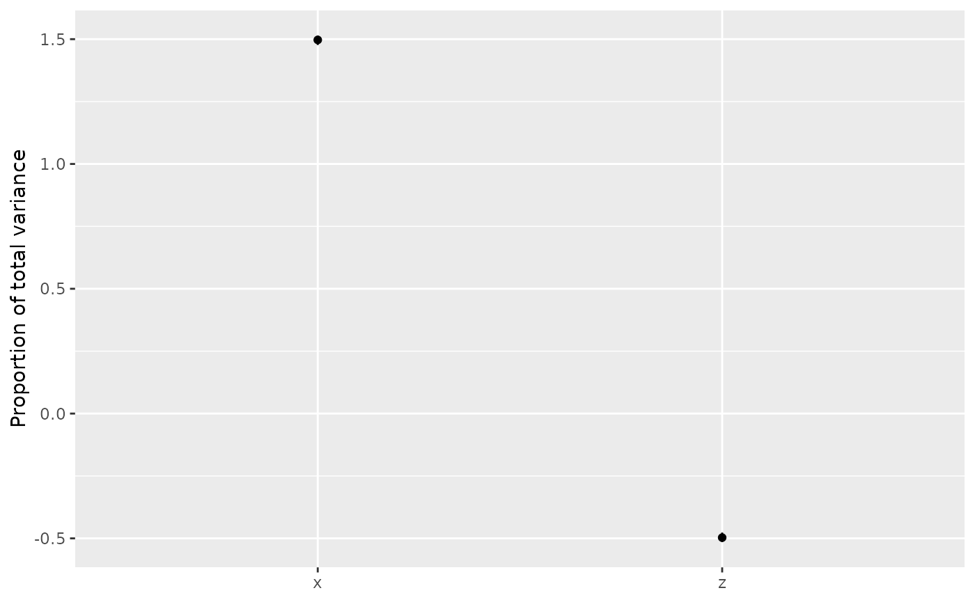

Their negative covariance reduces the variance of their sum. Accounting for this covariance gives x a share of 1.5 and z a share of -0.5. Proportions can therefore exceed one or be negative. They are undefined (NA) when the total variance is zero.