Smooth trends and repeated measurements with glmmTMB • gratia

A smooth describes a relationship without requiring it to be linear. glmmTMB can estimate these relationships alongside its other model components, and gratia can now extract and display their effects. The examples below ask how annual river flow changes over time and how plants respond to increasing carbon dioxide concentration. The second example also accounts for measurements on the same plant.

This article needs the optional package glmmTMB, with support for mgcv::s() terms; the examples require glmmTMB 1.1.15.2 or later and mgcv 1.9-4. Smooth fitting remains experimental in glmmTMB. Its fitting documentation recommends REML = TRUE. Use an unqualified s() in the formula after attaching mgcv, rather than replacing the smooth with an unpenalised spline basis. The smoothing penalty is estimated during fitting.

library("mgcv")
library("glmmTMB")
library("gratia")
library("ggplot2")

How did the mean annual flow of the Nile change?

The Nile data contain 100 annual flow measurements at Aswan from 1871 to 1970, measured in units of 10^8 cubic metres. The question here is descriptive: what broad change in mean flow is supported by these observations? We adapt the smooth example in the glmmTMB documentation, name the variables year and flow, and fit the same spline with mgcv for comparison.

nile <- data.frame(
  year = as.numeric(time(Nile)),
  flow = as.numeric(Nile)
)
ggplot(nile, aes(year, flow)) +
  geom_point() +
  labs(x = "Year", y = expression(Annual ~ flow ~ (10^8 ~ m^3)))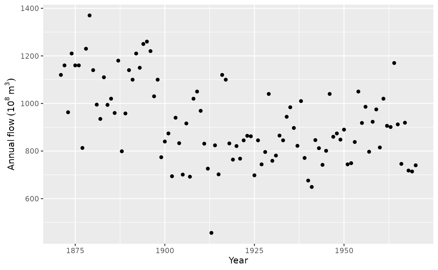

Annual flow is continuous. A Gaussian model is a reasonable starting point for departures around a smooth mean, provided its residual spread is reasonably stable. The observations are a time series, so independence needs checking; year appearing in a smooth does not itself model residual serial dependence.

nile_gam <- gam(flow ~ s(year, k = 10), data = nile, method = "REML")
nile_tmb <- glmmTMB(flow ~ s(year, k = 10), data = nile,
  family = gaussian(), REML = TRUE, start = list(theta = 5))
summary(nile_tmb)
#>  Family: gaussian  ( identity )
#> Formula:          flow ~ s(year, k = 10)
#> Data: nile
#> 
#>       AIC       BIC    logLik -2*log(L)  df.resid 
#>    1265.7    1276.1    -628.8    1257.7        96 
#> 
#> Random effects:
#> 
#> Conditional model:
#>  Groups   Name   Variance Std.Dev.
#>  dummy    dummy1 81075    284.7   
#>  Residual        19000    137.8   
#> Number of obs: 100, groups:  dummy, 1
#> 
#> Dispersion estimate for gaussian family (sigma^2): 1.9e+04 
#> 
#> Conditional model:
#>             Estimate Std. Error z value Pr(>|z|)    
#> (Intercept)   919.35      13.78   66.70   <2e-16 ***
#> s(year)1       99.30      86.34    1.15     0.25    
#> ---
#> Signif. codes:  0 '***' 0.001 '**' 0.01 '*' 0.05 '.' 0.1 ' ' 1

k = 10 sets the size of the available spline basis, rather than fixing ten effective degrees of freedom. The fitted penalty discourages unnecessary wiggliness. start follows the package’s Nile example and supplies an initial log standard deviation for the spline’s random coefficients; it does not fix their fitted variance. The dummy random effect in the printed summary is part of the spline representation, not an additional sampled group.

Extract the trend and read its uncertainty

smooths(nile_tmb)
#> [1] "s(year)"
head(smooth_coefs(nile_tmb, select = "s(year)"))
#>   s(year).1   s(year).2   s(year).3   s(year).4   s(year).5   s(year).6 
#>   18.174609 -115.231114   -2.991595  -24.387354  -15.572794   13.125102
trend <- smooth_estimates(nile_tmb, select = "s(year)",
  interval = "credible")
head(trend)
#> # A tibble: 6 × 9
#>   .smooth .type .by   .estimate   .se  year .crit .lower_ci .upper_ci
#>   <chr>   <chr> <chr>     <dbl> <dbl> <dbl> <dbl>     <dbl>     <dbl>
#> 1 s(year) TPRS  NA         226.  49.6  1871  1.96      129.      323.
#> 2 s(year) TPRS  NA         220.  46.3  1872  1.96      129.      311.
#> 3 s(year) TPRS  NA         214.  43.2  1873  1.96      129.      299.
#> 4 s(year) TPRS  NA         208.  40.4  1874  1.96      129.      287.
#> 5 s(year) TPRS  NA         202.  37.8  1875  1.96      128.      276.
#> 6 s(year) TPRS  NA         196.  35.6  1876  1.96      127.      266.
draw(trend, xlab = "Year", ylab = expression(Flow ~ contribution ~ (10^8 ~ m^3)))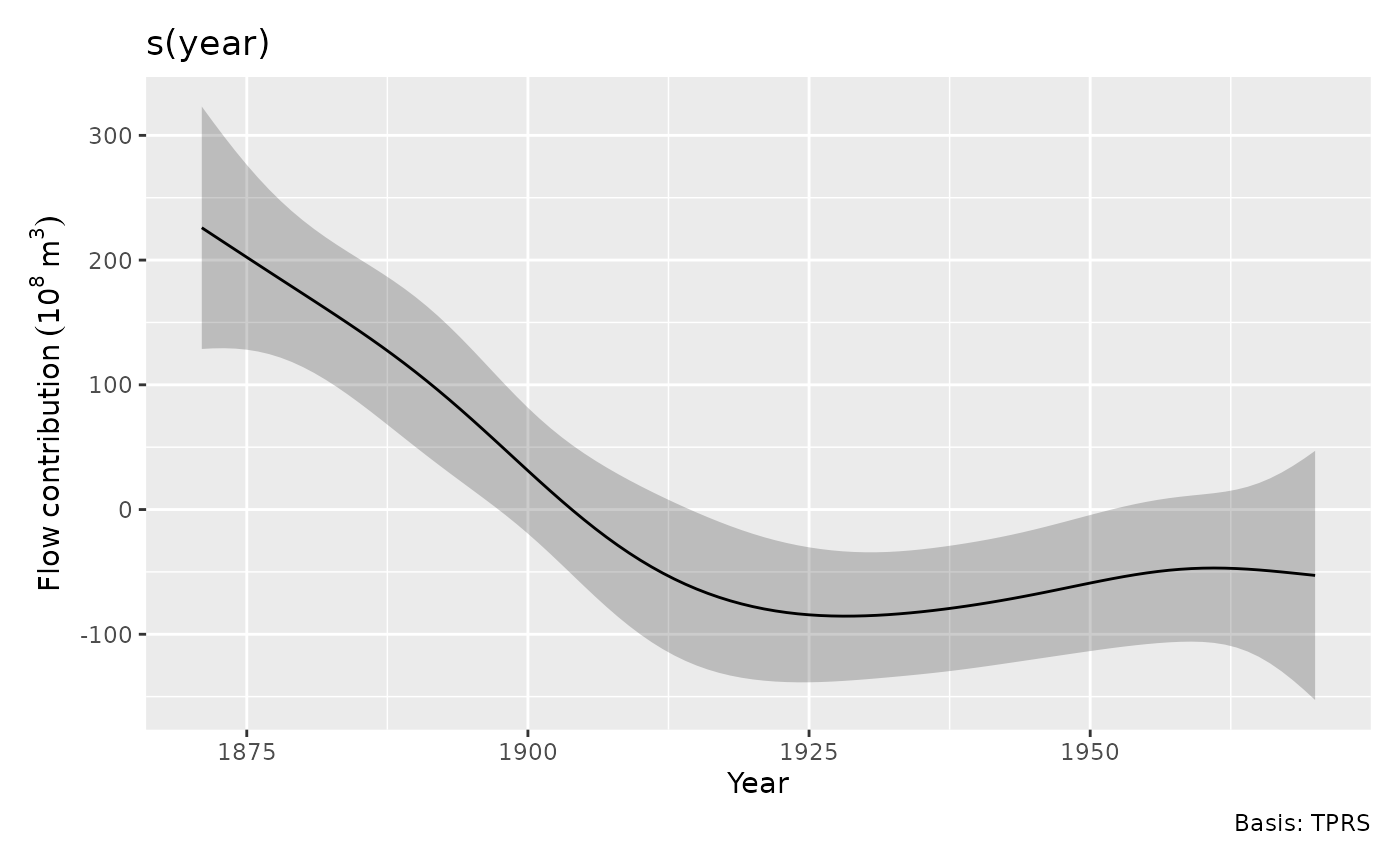

The curve is the smooth’s contribution relative to its centring constraint, not the full expected flow. Positive values indicate flow above the fitted intercept. The broad decline from the late nineteenth century to the early twentieth century is much clearer than the small subsequent undulations. The shaded region concerns uncertainty in the fitted mean contribution; it does not describe the spread of individual annual observations.

The default interval uses the joint TMB covariance, transformed back to the mgcv smooth coefficients. It includes covariance between fixed and fitted random coefficients. This is not mgcv’s frequentist covariance or its optional correction for uncertainty in smoothing parameters: frequentist = TRUE and unconditional = TRUE are unavailable for glmmTMB effects.

At any particular year a pointwise interval is useful. If the claim concerns the entire plotted trend, ask for a simultaneous band instead:

draw(nile_tmb, select = "s(year)", interval = "simultaneous",
  n = 120, n_sim = 3000, seed = 71,
  xlab = "Year", ylab = expression(Flow ~ contribution ~ (10^8 ~ m^3)))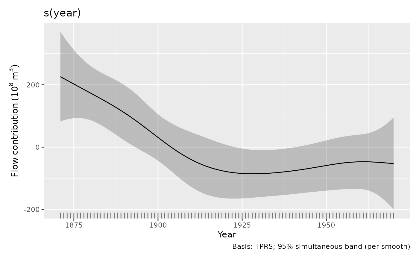

The wider band has approximate coverage over the finite evaluation grid of this smooth. It is not a prediction interval, and it does not claim joint coverage across all model terms. interval = "credible" is an alias for the pointwise "confidence" option. With mgcv models, smooth_estimates() also allows frequentist = TRUE; that changes the covariance used, rather than changing a pointwise statement into a simultaneous one. get_vcov() makes the chosen model covariance available for custom calculations.

For the full expected flow, add the intercept. Here the model has just one smooth and an identity link, so this gives a direct comparison with both packages’ predictions:

year_grid <- data.frame(year = seq(1871, 1970, length.out = 120))
full_trend <- smooth_estimates(nile_tmb, data = year_grid,
  interval = "credible")
full_trend$mean_flow <- full_trend$.estimate + unname(fixef(nile_tmb)$cond[1])
full_trend$lower <- full_trend$.lower_ci + unname(fixef(nile_tmb)$cond[1])
full_trend$upper <- full_trend$.upper_ci + unname(fixef(nile_tmb)$cond[1])
full_trend$mgcv_mean <- as.numeric(predict(nile_gam, newdata = year_grid))
ggplot(full_trend, aes(year, mean_flow)) +
  geom_point(data = nile, aes(y = flow), alpha = 0.5) +
  geom_ribbon(aes(ymin = lower, ymax = upper), alpha = 0.2) +
  geom_line() +
  geom_line(aes(y = mgcv_mean), colour = "steelblue", linetype = 2) +
  labs(x = "Year", y = expression(Annual ~ flow ~ (10^8 ~ m^3)),
    subtitle = "glmmTMB mean and interval; dashed blue line is the mgcv mean")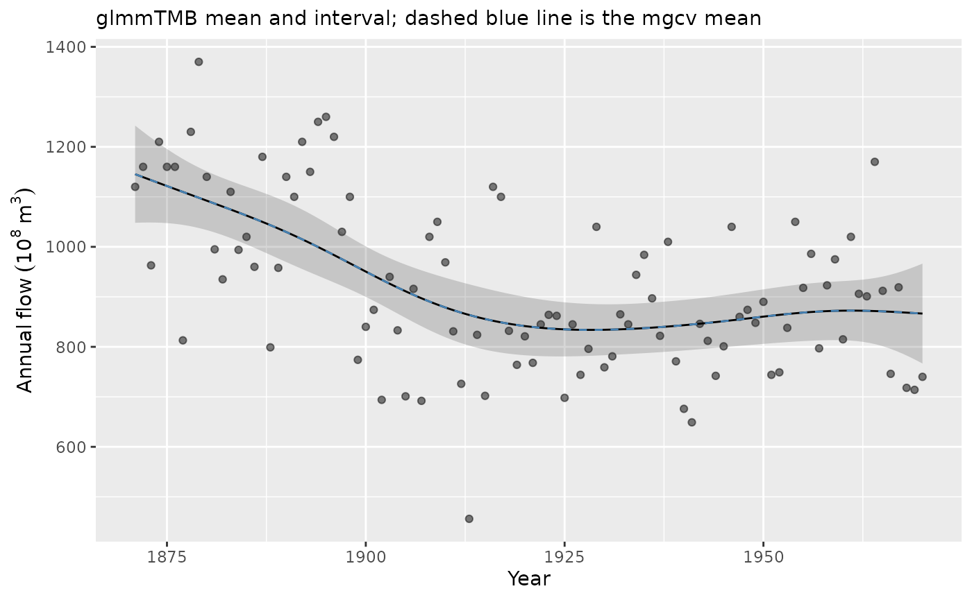

overall_uncertainty = TRUE, the default, includes uncertainty in the model constant in the smooth’s standard errors. Adding the intercept to the displayed values therefore gives appropriate mean intervals for this one-smooth model. For a model with several terms, adding only the intercept would leave out the other contributions; use predictions from the full model instead. The two mean curves almost coincide here because the models use the same Gaussian likelihood and spline penalty. Such agreement is not expected automatically for non-Gaussian fits or more complex random-effect structures.

For the mgcv fit, we can compare the two covariance choices at years of interest while leaving the estimated trend unchanged:

comparison_years <- data.frame(year = c(1880, 1920))
bayesian_effect <- smooth_estimates(nile_gam, data = comparison_years)
frequentist_effect <- smooth_estimates(nile_gam, data = comparison_years,
  frequentist = TRUE, interval = "confidence")
data.frame(year = comparison_years$year,
  contribution = bayesian_effect$.estimate,
  bayesian_se = bayesian_effect$.se,
  frequentist_se = frequentist_effect$.se)
#>   year contribution bayesian_se frequentist_se
#> 1 1880    172.99113    29.51978       28.36395
#> 2 1920    -77.82668    25.22793       22.21411
gam_covariance <- get_vcov(nile_gam, frequentist = TRUE)

The frequentist covariance concerns sampling variability of the penalised coefficient estimator with smoothing parameters held fixed. Smaller standard errors do not account for the bias introduced by penalisation. The default approximate Bayesian covariance is usually the useful starting point for smooth-effect intervals. The final line extracts the chosen covariance for custom calculations.

Does the fitted distribution explain variation around the trend?

appraise(nile_tmb, type = "pearson", method = "simulate",
  n_simulate = 100, seed = 72)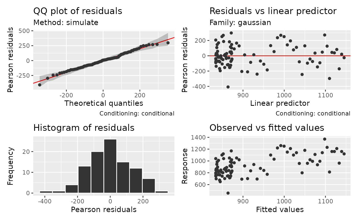

residual_correlation_plot(nile_tmb, type = "pearson", lag_max = 15)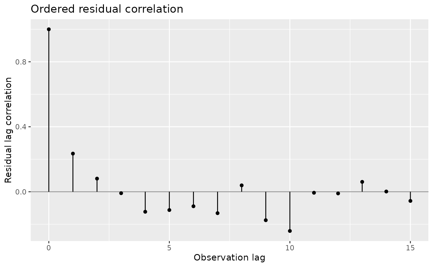

The panel uses glmmTMB’s native Pearson residuals. For this Gaussian fit they remain on the scale of the flow response, rather than standard-normal scores. Simulated QQ references hold the fitted smooth fixed and generate new annual responses. They check the response distribution under this fitted model; they do not refit the trend. The separate autocorrelation plot asks whether successive departures still resemble one another. Its correlations describe ordered residual structure, with no significance bands that assume independent residuals. Lags are observation positions; here each position corresponds to one year.

Most of the QQ points follow their simulated reference, with the lowest-flow observation standing out in the lower tail. The serial-correlation plot checks whether neighbouring years have similar departures from that distribution.

The residual correlation at lag one is about 0.24, with much smaller correlation at lag two. Some adjacent-year structure remains after removing the smooth trend. A time-series model can represent that remaining correlation when estimating trend uncertainty. The smooth describes a broad decline in mean flow, while the residual check identifies variation that its independent Gaussian errors leave unexplained. See Choosing diagnostic references for checks of dependence and for the distinction between holding effects fixed, drawing their uncertainty and simulating new effects.

Do repeated measurements change how we read plant responses?

The CO2 experiment recorded carbon dioxide uptake by twelve plants of Echinochloa crus-galli at seven concentrations. Plants came from Quebec or Mississippi and received chilled or nonchilled treatment. See ?datasets::CO2 for the experiment and units. Uptake is positive, and a Gamma model with a log link allows its residual variance to grow with the mean. Measurements from one plant share individual characteristics. The 84 measurements provide only twelve independently treated plants.

We use a shared smooth response to concentration, an origin-by-treatment interaction, and plant-specific intercepts and slopes. These slopes allow individual plants to differ in their response to concentration without assuming that the population response itself is linear.

plant <- as.data.frame(CO2)
plant$Plant <- factor(plant$Plant, ordered = FALSE)
plant$log_conc <- log(plant$conc) - mean(log(plant$conc))
plant_tmb <- glmmTMB(
  uptake ~ Type * Treatment + s(log_conc, k = 5) + (1 + log_conc | Plant),
  data = plant, family = Gamma(link = "log"), REML = TRUE)
summary(plant_tmb)
#>  Family: Gamma  ( log )
#> Formula:          
#> uptake ~ Type * Treatment + s(log_conc, k = 5) + (1 + log_conc |      Plant)
#> Data: plant
#> 
#>       AIC       BIC    logLik -2*log(L)  df.resid 
#>     454.1     478.4    -217.0     434.1        74 
#> 
#> Random effects:
#> 
#> Conditional model:
#>  Groups Name        Variance Std.Dev. Corr 
#>  dummy  dummy1      0.532393 0.72965       
#>  Plant  (Intercept) 0.013376 0.11565       
#>         log_conc    0.007544 0.08685  0.36 
#> Number of obs: 84, groups:  Plant, 12; dummy, 1
#> 
#> Dispersion estimate for Gamma family (sigma^2): 0.0067 
#> 
#> Conditional model:
#>                                  Estimate Std. Error z value Pr(>|z|)    
#> (Intercept)                       3.50826    0.06743   52.03  < 2e-16 ***
#> TypeMississippi                  -0.31784    0.09327   -3.41 0.000655 ***
#> Treatmentchilled                 -0.13966    0.09931   -1.41 0.159638    
#> TypeMississippi:Treatmentchilled -0.27192    0.18888   -1.44 0.149972    
#> s(log_conc)1                      0.46392    0.04158   11.16  < 2e-16 ***
#> ---
#> Signif. codes:  0 '***' 0.001 '**' 0.01 '*' 0.05 '.' 0.1 ' ' 1

For non-Gaussian responses, glmmTMB recommends simulations for the intended design to check REML estimates and interval coverage.

The centred log concentration improves the interpretation of plant intercepts: they apply at the geometric mean concentration. The shared curve represents rapid change at low concentrations and slower change at high concentrations. The treatment interaction allows its shift in log mean uptake to differ by origin. With only three plants in each origin-treatment combination, the treatment estimates remain uncertain.

draw(plant_tmb, ncol = 2)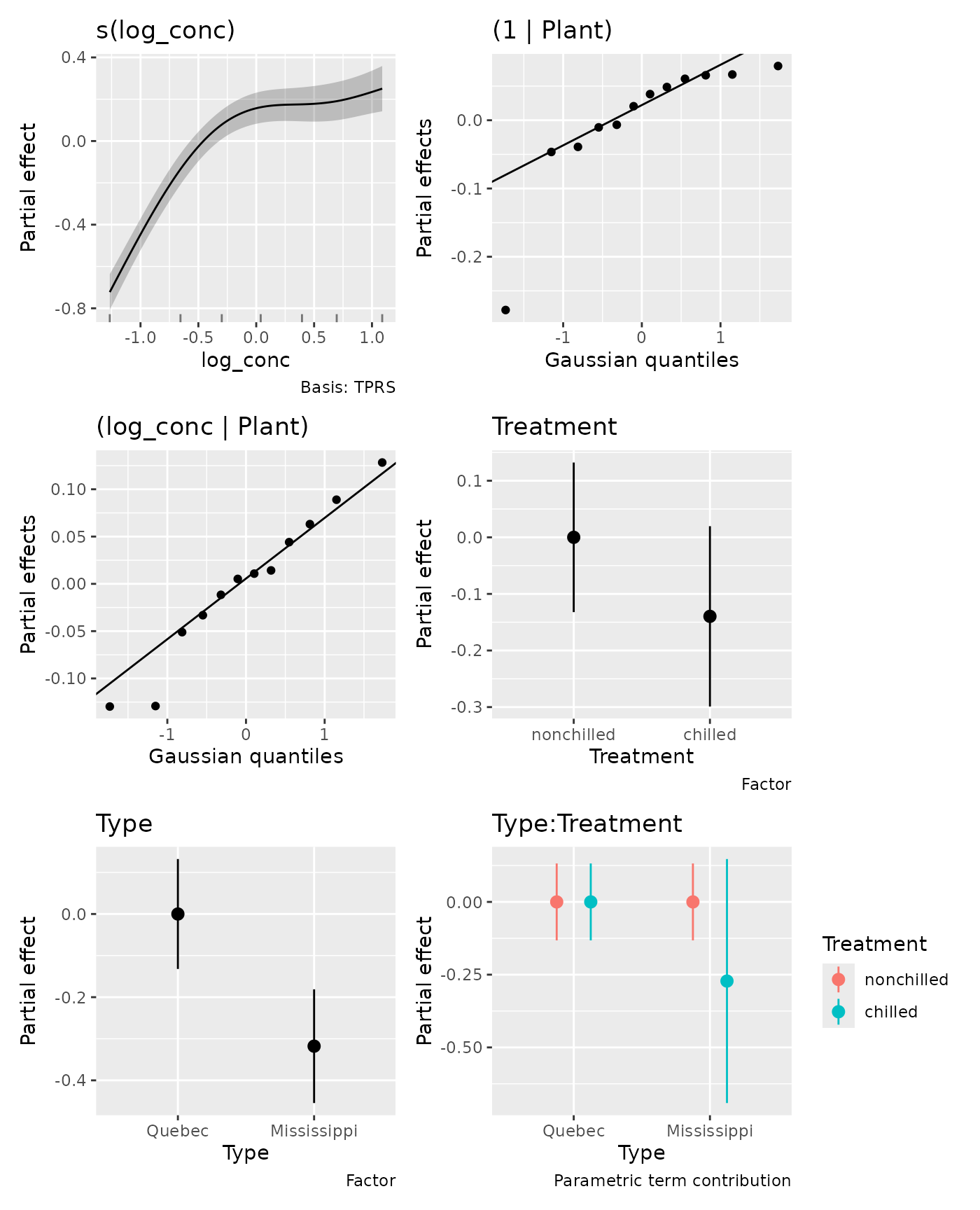

draw() includes smooths, native random effects and parametric effects by default. The Gaussian QQ panels for plant intercepts and slopes show fitted plant deviations, not response residuals. The random coefficients that encode the spline are excluded from these panels. parametric = FALSE omits parametric panels; an explicit select draws only selected effects unless parametric = TRUE is also supplied.

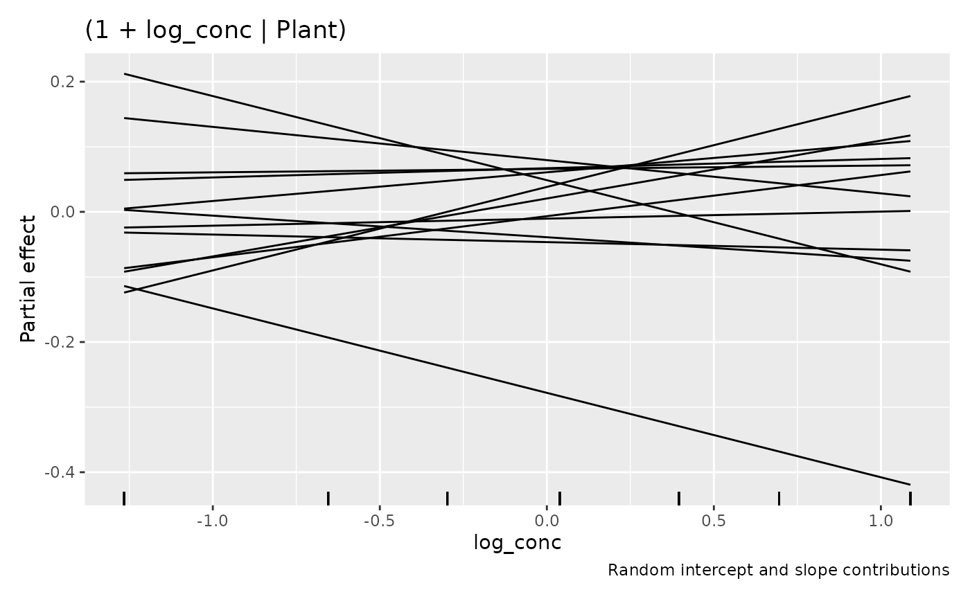
draw(plant_tmb, select = c("(1 | Plant)", "(log_conc | Plant)"),
  ranef_lines = TRUE)

These lines are each plant’s random contribution b_{0j} + x b_{1j} on the log scale. They do not include the shared curve or treatment means and have no uncertainty bands. This display requires a simple numeric intercept-slope pair from the same formula term. Multiple slopes, transformed or factor slopes, and structured covariance terms retain separate QQ panels.

The interaction deserves a focused view rather than interpreting two main effects separately:

parametric_terms(plant_tmb)
#>             Type        Treatment   Type:Treatment 
#>           "Type"      "Treatment" "Type:Treatment"
draw(parametric_effects(plant_tmb, terms = "Type:Treatment"))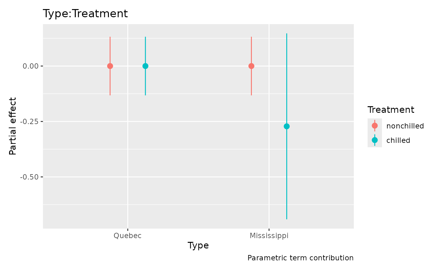

These are contrast-coded partial contributions on the log scale. Contrast coding gives the reference category a zero contribution; full predictions add the intercept and the other model terms. Parametric intervals now include intercept uncertainty and its covariance with the term by default; use overall_uncertainty = FALSE for uncertainty in the term alone. The estimated partial contributions do not change. Full predictions combine all terms:

plant$expected <- as.numeric(predict(plant_tmb, type = "response"))
ggplot(plant, aes(conc, uptake, group = Plant, colour = Treatment)) +
  geom_point() +
  geom_line(aes(y = expected)) +
  facet_wrap(~ Type) +
  labs(x = "Carbon dioxide concentration (mL/L)",
    y = expression(CO[2] ~ uptake ~ (mu * mol ~ m^{-2} ~ s^{-1})))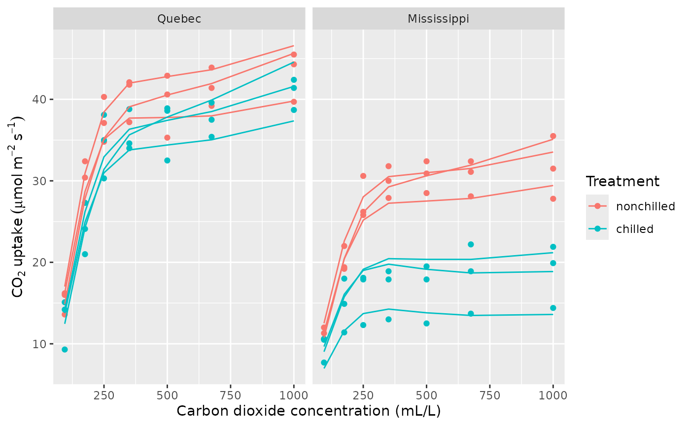

The curves describe these observed plants, including their fitted deviations. They are not marginal mean curves for a new plant. The Gamma model and common nonlinear shape are working assumptions that should be checked:

appraise(plant_tmb, type = "quantile", seed = 73)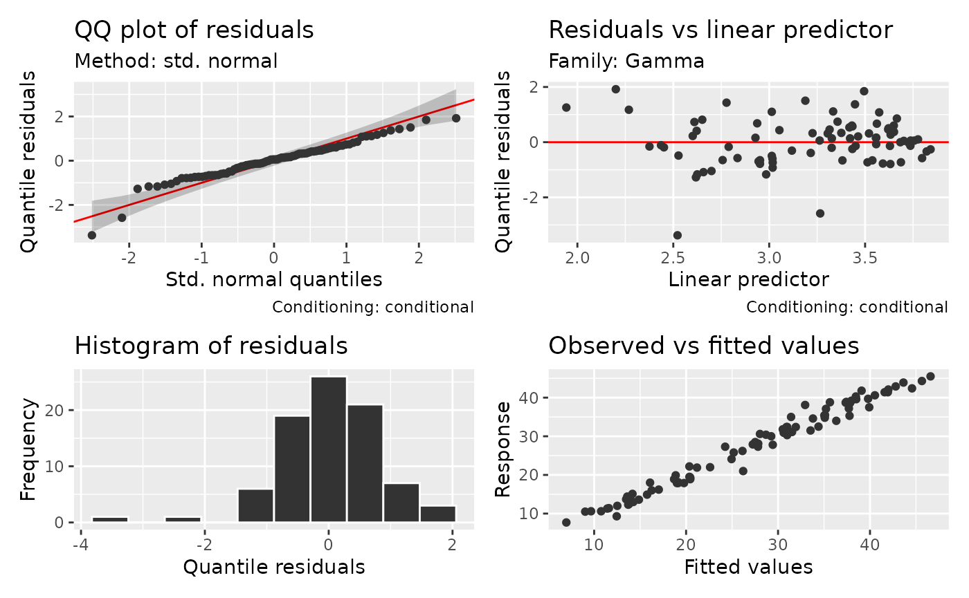

The lowest quantile score stands out below the normal reference: one measurement is substantially lower than its fitted distribution would typically produce. Inspect that observation and the fitted curve for its plant to decide whether its individual concentration response needs more flexibility. Read smooth effects, interactions and surfaces explores more flexible plant-specific curves.

A conditional check holds the fitted plant effects and smooth fixed. Quantile residuals use a fixed standard-normal reference to assess the distribution of individual scores conditional on those effects; the reference does not preserve dependence between scores. A marginal check instead draws new plant effects and new spline random coefficients with glmmTMB’s simulator. It therefore checks a broader distribution than that of new plants around a fixed shared concentration curve. The same scope applies to marginal posterior predictive checks. Conditional posterior predictive checks draw uncertainty in fitted coefficients and effects together. These answer different questions; see Choosing diagnostic references. Partial-residual overlays are not supported for glmmTMB smooth plots. For supported response families, model parts and current limitations, consult ?"glmmTMB-methods". Multiple linear predictors retain model-wide smooth selection and identify the conditional, zero-inflation or dispersion model in their plot subtitles; constant dispersion alone does not add these subtitles.

gratia cannot make a smooth type available if glmmTMB cannot fit it. Effects require the stored smooth and random-effect information; unsupported structures with several penalties, models that fix or share joint parameters through map, and rank-deficient smooth models give explicit errors. For a GAM that does not require glmmTMB’s additional model components, mgcv offers a broader range of spline constructions.