Posterior predictive checks and approximate leave-one-out comparisons

Gavin L. Simpson

Gratia can prepare posterior predictive checks for bayesplot and observation log likelihoods for loo. Both packages are optional: install them to use their methods. log_lik() itself needs neither package. The existing appraise() and posterior_predictive_plot() functions also work without them.

Some bayesplot plots, including error_binned and the LOO-PIT plots, also require bayesplot’s optional rstantools package; install it with install.packages("rstantools") to use those plots.

library("mgcv")
#> Loading required package: nlme
#> This is mgcv 1.9-4. For overview type '?mgcv'.
library("gratia")
set.seed(278)
dat <- data.frame(x = runif(100, -1, 1))
dat$y <- rpois(nrow(dat), exp(.3 + sin(3 * dat$x)))
linear <- gam(y ~ x, data = dat, family = poisson(), method = "REML")
smooth <- gam(y ~ s(x, k = 7), data = dat, family = poisson(), method = "REML")

Check replicated responses

For each coefficient draw, a posterior predictive check generates another response at every fitting observation. The variation between these replicated data sets includes coefficient uncertainty and response variation.

bayesplot::pp_check(smooth, type = "dens_overlay", n_draws = 20, seed = 42)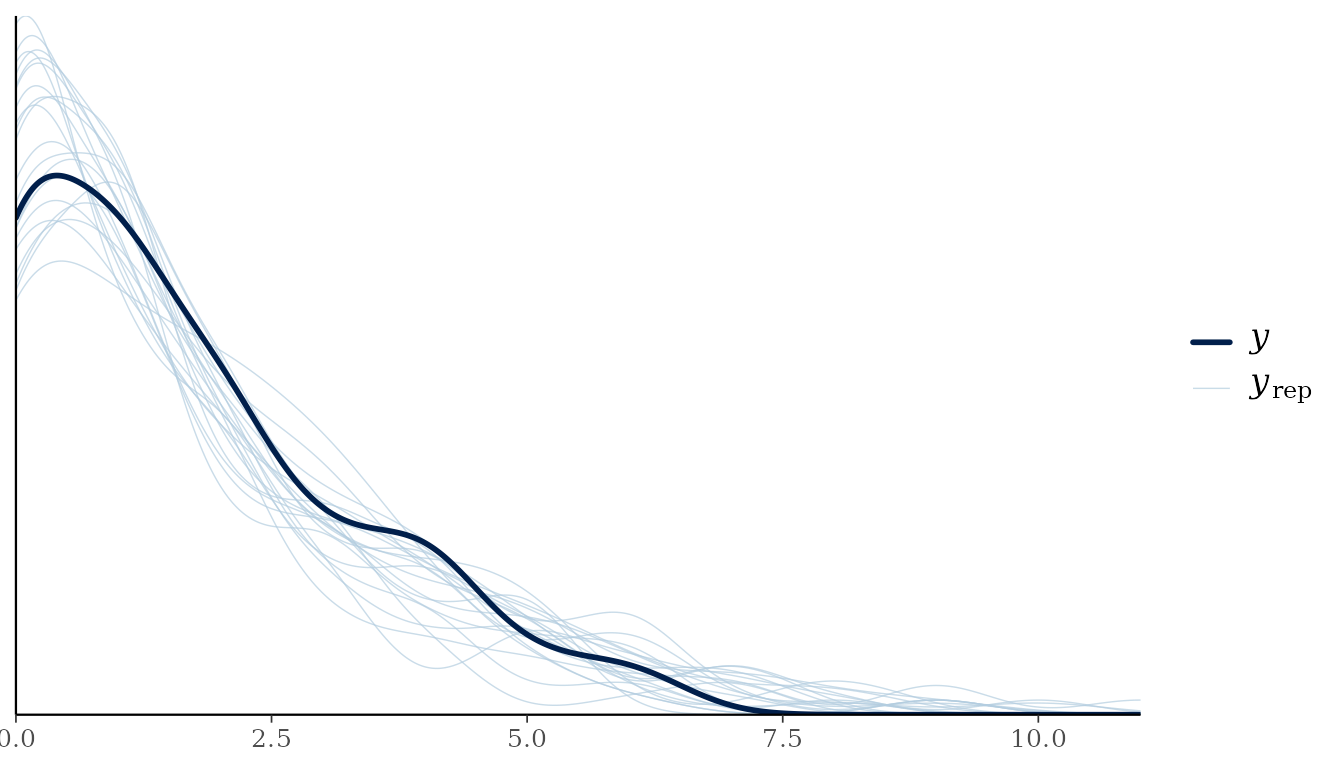

bayesplot::pp_check(smooth, type = "stat", stat = "sd", n_draws = 500, seed = 42)
#> `stat_bin()` using `bins = 30`. Pick better value `binwidth`.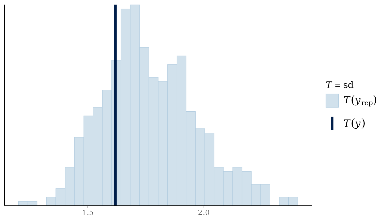

The first plot compares the observed response distribution with replicated distributions. The second checks whether their standard deviations cover the observed standard deviation. Other bayesplot statistics can be supplied through stat, including a function such as function(y) mean(y == 0) for the proportion of zeroes. To display predictions alone, use prefix = "ppd".

Grouped plots accept a fitting-frame variable name or a vector in fitting-row order. A vector is useful when the grouping variable was not used in the model.

bayesplot::pp_check(smooth, type = "stat_grouped", stat = "mean", n_draws = 500,
  group = factor(dat$x > 0, labels = c("negative x", "positive x")), seed = 42)
#> Note: in most cases the default test statistic 'mean' is too weak to detect anything of interest.
#> `stat_bin()` using `bins = 30`. Pick better value `binwidth`.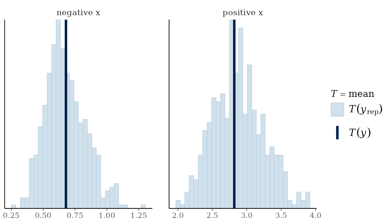

Missing fitting rows are omitted consistently from responses and covariates. Binomial checks use success counts and fitted trial counts; gratia’s own posterior predictive plots use proportions. Multivariate and grouped-family models require response, for example "response1" or "component2". These selections keep distinct responses and observation families from being pooled. For gamm/gamm4 fits, conditioning retains its existing gratia meaning.

Evaluate observed-response log likelihoods

log_lik() holds each response at its observed value and evaluates its log density or log probability mass at each coefficient draw. Rows are posterior draws and columns are retained fitting observations. For example, a Poisson entry is dpois(y[i], lambda = mu[s, i], log = TRUE).

ll <- gratia::log_lik(smooth, n_draws = 2000, seed = 42)
dim(ll)
#> [1] 2000  100
head(attr(ll, "observation"))
#> [1] 1 2 3 4 5 6
attr(ll, "gratia")
#> $method
#> [1] "gaussian"
#> 
#> $n_draws
#> [1] 2000
#> 
#> $chains
#> [1] 1
#> 
#> $approximation
#> [1] "Gaussian coefficient posterior approximation"
#> 
#> $fixed_parameters
#> [1] "Smoothing parameters and family parameters outside the coefficient vector remain at fitted values."
#> 
#> $unconditional
#> [1] FALSE
#> 
#> $posterior_correction
#> [1] FALSE

These values include the fitting likelihood’s normalising constants and weights, but exclude smoothing penalties. They differ from the single fitted log likelihood returned by stats::logLik(smooth), whose existing behaviour is unchanged. A multivariate-normal observation contributes a joint density for its complete response vector. Grouped-family rows use their respective family.

Compare predictive performance with loo

Loo uses importance weights to approximate the predictions obtained by leaving one observation out. Its elpd_loo estimate summarises expected log predictive density: larger values indicate better predictions on the same response scale and the same observations.

loo_linear <- loo::loo(linear, n_draws = 2000, seed = 42)
loo_smooth <- loo::loo(smooth, n_draws = 2000, seed = 42)
loo::loo_compare(loo_linear, loo_smooth)
#>   model elpd_diff se_diff p_worse diag_diff diag_elpd
#>  model2       0.0     0.0      NA                    
#>  model1     -14.0     4.2    1.00
loo::pareto_k_table(loo_smooth)
#> 
#> All Pareto k estimates are good (k < 0.7).

The methods return ordinary loo objects, so loo’s plotting, model-comparison and weighting tools are available. For an already extracted matrix of independent Gaussian coefficient draws, the equivalent calculation is loo::loo(ll, r_eff = 1). loo::waic(smooth, n_draws = 2000, seed = 42) also works. Model methods evaluate likelihoods one observation at a time, avoiding a full draws-by-observations matrix unless saved PSIS weights are requested.

Large Pareto-k values identify observations whose omission is difficult to approximate by reweighting the existing draws. Inspect these observations and loo’s warnings before relying on a comparison. Use explicit refits or a separate cross-validation analysis when reweighting is unreliable; these methods do not automatically refit models or perform moment matching.

LOO predictive plots use response simulations and importance weights from the same coefficient draws:

bayesplot::pp_check(smooth, type = "loo_pit_overlay", n_draws = 2000, seed = 42)
#> NOTE: The kernel density estimate assumes continuous observations and is not
#> optimal for discrete observations.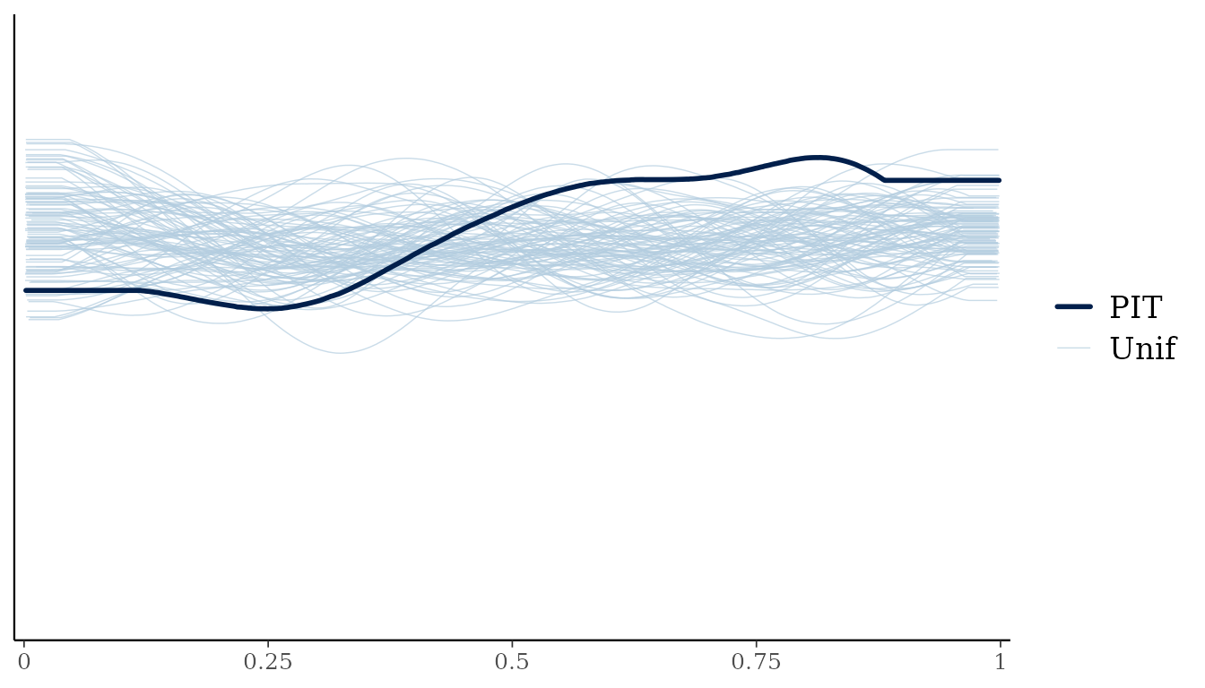

Understand the posterior approximation

By default, gratia draws coefficients jointly from mgcv’s Gaussian approximation. For a distributional GAM, this includes coefficients for each distribution parameter. For multivariate-normal likelihoods, it also includes the fitted precision-matrix coefficients. Scale, shape and other parameters outside the coefficient vector stay at fitted values, as do smoothing parameters.

This is a conditional approximation, rather than a procedure that re-estimates every parameter for every omitted observation. unconditional = TRUE can use mgcv’s corrected coefficient covariance when available, but it does not draw those other parameters jointly. PSIS calculations do not correct the Gaussian approximation, and small Pareto-k values do not establish its accuracy.

# Extra sampler arguments are kept separate from loo and plotting arguments.
loo::loo(smooth, n_draws = 2000, seed = 42,
  sampling_args = list(unconditional = TRUE))
bayesplot::pp_check(smooth, n_draws = 50, seed = 42,
  sampling_args = list(unconditional = TRUE))

# Four chains share the total retained count, with separate burn-in.
loo::loo(smooth, n_draws = 2000, seed = 42,
  sampling_args = list(method = "mh", chains = 4, burnin = 1000))

For supplied coefficient draws, use method = "user", draws = B in log_lik(), or place those arguments in sampling_args for loo and bayesplot. LOO uses the chain and iteration mapping stored by gratia’s samplers. For an unlabelled matrix, supply chain_id or an explicit r_eff; gratia cannot infer chain boundaries from its dimensions. A supplied chain_id must agree with stored metadata. Bootstrap coefficient samples do not become posterior draws by passing them to this interface.

n_draws is the total retained count, so 2,000 draws over four chains retains 500 draws per chain. Likelihood and LOO/WAIC wrappers default to 4,000 draws; bayesplot uses 50 for ordinary checks and 4,000 for leave-one-out plots. Supplied matrices determine their own count and chains. These wrappers reject the obsolete n argument, and inactive sampler controls produce errors. Use diagnostics = TRUE directly in log_lik(), or in sampling_args for LOO and bayesplot, to retain coefficient diagnostics. The likelihood matrix also supports as_mcmc_draws() for diagnostics of its observation-wise log densities.

Likelihood and LOO methods initially cover independent GAM/BAM responses. They exclude residual-correlated BAMs, full gamm/gamm4 fits, quasi families, Cox partial likelihoods and censored observation processes. Supported ordinary posterior predictive checks retain their existing model coverage. With random-effect smooths, observation-level LOO predicts further observations in the fitted groups; it does not leave out entire groups.

The reproducible script inst/validation/loo-refits.R compares representative Gaussian, Poisson and binomial PSIS results with explicit leave-one-out refits. It distinguishes refits that hold smoothing and nuisance parameters fixed from refits that re-estimate them.