Effects and diagnostics for glmmTMB models

Evaluate and plot the stored mgcv smooths in a glmmTMB fit. Coefficients and their joint covariance are transformed back to the constrained mgcv basis. Intervals use TMB's joint covariance, including fixed–random covariance; they are not mgcv frequentist or smoothness-corrected intervals.

Usage

# S3 method for class 'glmmTMB'
qq_plot(model, ..., method = NULL, type = NULL, conditioning = NULL)

# S3 method for class 'glmmTMB'
worm_plot(model, ..., method = NULL, type = NULL, conditioning = NULL)

# S3 method for class 'glmmTMB'
appraise(model, ..., method = NULL, type = NULL, conditioning = NULL)

# S3 method for class 'glmmTMB'
parametric_terms(model, ...)

# S3 method for class 'glmmTMB'
parametric_effects(
  object,
  terms = NULL,
  ...,
  unconditional = FALSE,
  frequentist = FALSE
)

# S3 method for class 'glmmTMB'
smooths(object, ...)

# S3 method for class 'glmmTMB'
get_smooths_by_id(object, id, ...)

# S3 method for class 'glmmTMB'
smooth_estimates(object, ..., unconditional = FALSE, frequentist = FALSE)

# S3 method for class 'glmmTMB'
smooth_coefs(object, select, ...)

# S3 method for class 'glmmTMB'
draw(
  object,
  ...,
  parametric = NULL,
  residuals = FALSE,
  unconditional = FALSE,
  frequentist = FALSE,
  ranef_lines = FALSE,
  envir = NULL
)

Arguments

...

Arguments passed to the corresponding gratia method.

method

QQ method; NULL selects "simulate" for traditional residuals.

type

Residual type: "pearson", "response", "deviance", "pit", "quantile", or "dharma", when available for the family. The default is Pearson for conditional checks and response residuals for marginal checks.

conditioning

character or NULL; "conditional" (default) or "marginal"; see diagnostic_support.

object, model

A fitted glmmTMB model.

terms

Character vector selecting parametric terms, as returned by parametric_terms(). Later predictors append .1, .2, etc.

unconditional, frequentist

Must be FALSE; mgcv-specific covariance alternatives are not available.

id

Integer positions of smooths across all linear predictors.

select

Smooth or native random-effect coefficient selection, across all linear predictors. Numeric indices select smooths first, then native random coefficients. Native labels have the form (1 | g) and (x | g); later predictors append .1, .2, etc. smooth_estimates() and smooth_coefs() select smooths only.

parametric

Include parametric effect plots? NULL follows draw.gam(): include them unless select is supplied. Use terms to choose parametric terms, and parametric = FALSE to omit them.

residuals

Must be FALSE; partial residual overlays are not supported.

ranef_lines

Logical; replace QQ plots for a simple native random intercept and numeric slope term, (1 + x | g), with one panel of lines showing b[0,g] + x * b[1,g]? Defaults to FALSE. Both coefficients must be selected. Multiple slopes, interactions, factor slopes, transformed slopes and structured covariance terms retain separate QQ plots.

envir

Optional environment for evaluating model covariates.

Value

Smooth estimates, coefficients, or plots, as for the GAM methods. All smooths, native random effects and parametric terms are plotted by default, as for draw.gam(). Smooths in later linear predictors use mgcv-style labels such as s.1(x) and s.2(x). Predictor order is conditional, zero-inflation (if present), then dispersion (if present). Use smooths(object) and select to select individual smooths. For models with multiple linear predictors, smooth subtitles identify the "Conditional model", "Zero-inflation model" or "Dispersion model", consistently with native random-effect panels. Constant dispersion alone does not trigger these subtitles. names(draw(object, wrap = FALSE, parametric = FALSE)) also lists native random-effect coefficient panels.

Details

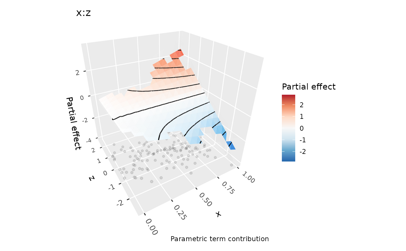
Smooth support requires stored smooth and random-effect metadata. Unsupported multi-penalty structures, mapped joint parameters and rank-deficient smooth models give errors. Factor-by and tensor smooth availability is determined by glmmTMB; gratia does not expand the smooth types glmmTMB can fit. Use draw(model, surface = "3d", ci_3d = TRUE) for interval surfaces on smooths and numeric parametric interactions in any linear predictor. ci_3d_alpha and ci_3d_col control their opacity and fill colour.

Parametric effects use fitted contrast coding and exclude smooth null-space coefficients. Their intervals include uncertainty in the intercept of their own linear predictor by default, as for GAMs. overall_uncertainty = FALSE gives term-only intervals. Models without smooths are also supported.

Native random effects use one Gaussian QQ panel per coefficient type and grouping factor, matching mgcv random-effect smooth plots. The internal random effects representing smooths are excluded from these panels. With ranef_lines = TRUE, eligible intercept-slope pairs use a common grid over the fitting range of the numeric covariate, or its supplied data values. Lines show random contributions only, without population-level terms or uncertainty bands. Different formula terms are never combined.

Diagnostics use native Pearson residuals by default. QQ simulations hold fitted smooths and grouping effects fixed and draw new responses; no refitting is performed. Supported response families are Gaussian, Poisson, binomial, nbinom1/2, beta, Gamma/ziGamma, Tweedie, lognormal, and zero-truncated Poisson/nbinom1/2, including applicable zero-inflation or hurdle mixtures and varying dispersion. Truncated nbinom1 currently requires type = "response" because glmmTMB does not supply its Pearson residuals. Other unavailable residual types fail explicitly. Supported fitted response distributions also provide randomized PIT/quantile residuals and inverse-CDF QQ references, including their zero-inflation and truncation probabilities. Posterior predictive checks draw coefficients and fitted random effects together from their approximate posterior. See posterior_predictive_plot() for how covariance and other family parameters are treated. Marginal checks simulate new effects using glmmTMB's response generator. If marginal CDFs are not analytic, residual checks use a shared sample of simulations to calculate moments and ranks. See diagnostic_support for conditioning choices and remaining limitations.

Examples

if (requireNamespace("glmmTMB", quietly = TRUE)) {
  library("mgcv")
  set.seed(42)
  d <- data.frame(x = runif(150))
  d$y <- sin(6 * d$x) + rnorm(150, sd = 0.2)
  m <- glmmTMB::glmmTMB(y ~ s(x, k = 8), data = d, REML = TRUE)
  n_smooths(m) # one smooth term
  draw(m)
  appraise(m, seed = 42)

  # Parametric terms and native random intercepts and slopes
  d$z <- rnorm(150)
  d$g <- factor(rep(seq_len(10), each = 15))
  d$y <- d$y + 0.5 * d$z + rnorm(10)[d$g] + rnorm(10)[d$g] * d$z
  mixed <- glmmTMB::glmmTMB(y ~ z + s(x, k = 8) + (1 + z | g),
    data = d, REML = TRUE)
  draw(mixed) # separate QQ panels for intercepts and slopes
  draw(mixed, ranef_lines = TRUE) # random contributions only
  if (requireNamespace("ggcube", quietly = TRUE)) {
    interaction <- glmmTMB::glmmTMB(y ~ x:z, data = d)
    draw(interaction, surface = "3d", ci_3d = TRUE, n_2d = 15)
  }
}