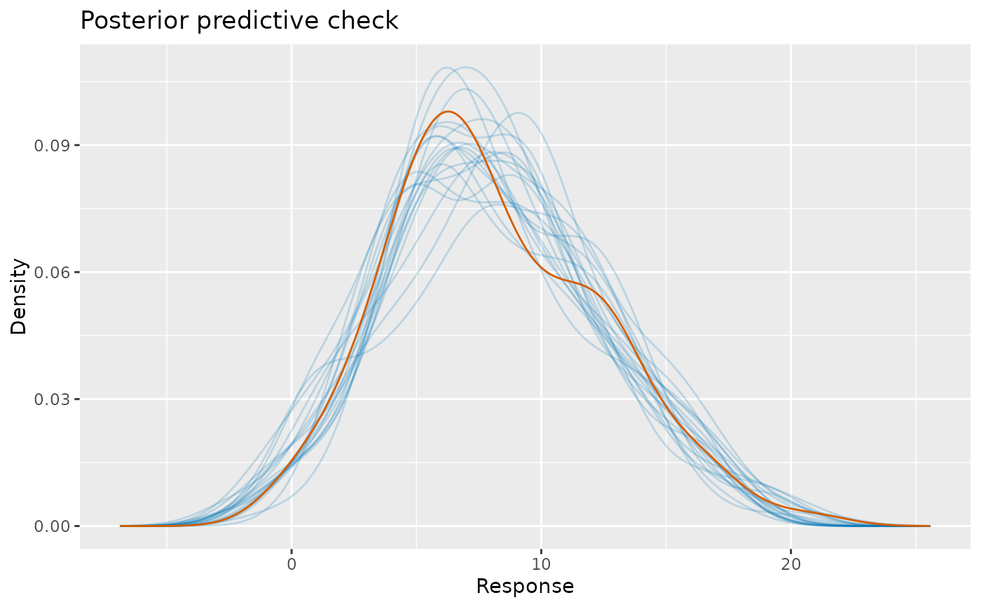
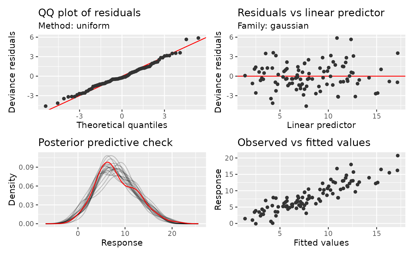
Posterior predictive check of the response distribution

Compare the observed response distribution with replicated data sets drawn from the approximate posterior predictive distribution of a fitted model.

Usage

posterior_predictive_plot(
  model,
  n = 50,
  seed = NULL,
  observed_col = "#D55E00",
  replicated_col = "#0072B2",
  replicated_alpha = NULL,
  xlab = NULL,
  ylab = NULL,
  title = "Posterior predictive check",
  subtitle = NULL,
  caption = NULL,
  level = 0.9,
  conditioning = NULL,
  scalable = NULL,
  scalable_threshold = 10000L,
  batch_size = 10L,
  ...
)

Arguments

model

a fitted model with a posterior response sampler.

n

positive integer; number of replicated data sets to draw.

seed

numeric; optional random seed. With an explicit seed, the caller's random-number state is preserved.

observed_col, replicated_col

Deprecated; use gratia_theme_get() theme settings instead. Colours for the observed and replicated distributions, respectively. Standalone plots default to orange-red ("#D55E00") and blue ("#0072B2"). When called by appraise(), the check uses that function's line_col and ci_col instead.

replicated_alpha

Deprecated; use gratia_theme_get() theme settings instead. Numeric or NULL; opacity of replicated distributions. The default, NULL, uses 0.8 for discrete posterior median points and interval bars, and 0.2 for continuous density curves.

xlab

character or expression; label for the response axis.

ylab

character or expression; the label for the y axis. If not supplied, a suitable label will be generated.

title

character or expression; the title for the plot. See ggplot2::labs().

subtitle

character or expression; the subtitle for the plot. See ggplot2::labs().

caption

character or expression; the plot caption. See ggplot2::labs().

level

numeric; coverage of the equal-tailed posterior predictive intervals for discrete responses. Must be strictly between zero and one. Defaults to 0.9. Ignored for continuous density overlays.

conditioning

character or NULL; mixed-model conditioning mode.

scalable

logical or NULL; summarize posterior response draws on a common grid, using temporary disk storage instead of retaining all responses in memory. NULL enables this at scalable_threshold observations.

scalable_threshold

positive integer; observation count for automatic scalable plotting.

batch_size

positive integer; number of draws per processing batch. Batch boundaries do not alter seeded draws. Scalable discrete comparisons with more than 512 distinct response values aggregate probability into 512 shared equal-width bins to bound memory and plot size.

...

arguments passed to posterior_samples(), such as unconditional or mvn_method. For delta sdmTMB fits, component = "response", "binomial", or "positive" selects the complete response or a fitted component. Prediction at new data is not supported.

Value

A ggplot object. Its data contain the observed responses (.draw = 0) and posterior replicates (.draw > 0), indexed by .row and .parameter. Scalable plots instead retain density or probability summaries evaluated on the same grid for all draws.

Details

Mixed-model captions name the conditioning mode. Supply caption to replace this text, or caption = "" to omit it.

Each replicated data set includes uncertainty in the coefficients and random variation in the responses, at the covariate values used to fit the model. Linear models and GLMs draw coefficients from a Gaussian distribution with the estimated coefficient covariance, keeping dispersion at its fitted value. For GAMs that model several distribution parameters, all their coefficients are drawn together. Distribution parameters outside this coefficient vector remain at fitted values, including additional parameters of grouped-family components.

glmmTMB draws mean, zero-inflation and dispersion coefficients together with fitted random effects, using a Gaussian (Laplace) approximation to their posterior. Their covariance includes uncertainty from estimating the parameters that control random-effect covariance. For conditional checks, responses are generated using the drawn values of the fitted random effects. Given those values, their prior covariance is not needed to generate responses. Additional family parameters, such as Tweedie power, remain at fitted values. For marginal checks, coefficient draws include the same estimation uncertainty, but new random effects are generated using the fitted prior covariance. Thus these checks keep the covariance of new effects fixed while retaining its estimation uncertainty in the coefficient draws; they do not condition the coefficient posterior on fixed covariance parameters. sdmTMB draws parameters together from a Gaussian approximation, including fixed coefficients and random fields, and uses sdmTMB's response simulator to generate the complete response. These plots do not require an analytic residual distribution, so native simulated families such as Student-t and beta-binomial are available. SCAM models support ordinary and scalable predictive checks using transformed coefficient draws. Gaussian identity-link AR1 fits retain the fitted response correlation and the series boundaries stored in AR.start. Gaussian gamm and gamm4 models draw fixed and random effects together, keeping covariance parameters at fitted values; marginal checks draw new effects. For gamm fits estimated by penalized quasi-likelihood (PQL), the sampler uses the Gaussian approximation used in fitting and then generates responses from the fitted response family. This is supported only when the Gaussian working residuals are uncorrelated. Correlation in those working residuals does not specify a joint distribution for responses from the fitted family. gamm4 defaults to conditioning = "conditional", checking the full fitted mixed model while including uncertainty in fitted effects. Use the explicit "gam_component" option for the extracted GAM calculations. GJRM draws the final distributional coefficients jointly. These are approximate predictive checks; no refitting is performed.

Continuous responses use kernel density estimates with a common bandwidth derived from the observed responses and a shared evaluation grid. Discrete responses show observed empirical probability masses as points, alongside posterior medians and equal-tailed intervals across replicated data sets. Observed points, predicted points and intervals are placed at the actual response values on the horizontal axis. Binomial responses are compared as proportions, including models fitted to success and failure counts. Each fitting observation contributes equally to the empirical distribution. Response sampling follows the fitted family's interpretation of weights; see posterior_samples(). Factor-valued binomial observations retain one Bernoulli trial per observation, and native gaulss fitting weights do not change its response precision. Explicit GAM sampling weights override the defaults. Multivariate normal responses are shown in separate facets.

Excluded observations are omitted from both observed and replicated data. Responses remain on the scale used in fitting, including transformations in the response formula. Grouped families use separate component facets. Censored responses require a model of how censoring changes the generated observations and are not supported. Unsupported models or samplers produce an error; no alternative simulation method is substituted. Additional sampler limitations are described in posterior_samples().

See also

appraise(), posterior_samples()

Examples

load_mgcv()
dat <- data_sim("eg1", n = 100, seed = 2)
mod <- gam(y ~ s(x0) + s(x1) + s(x2) + s(x3),
  data = dat,
  method = "REML"
)
posterior_predictive_plot(mod, n = 20, seed = 42)

appraise(mod, ppcheck = TRUE, n_ppc = 20, seed = 42)