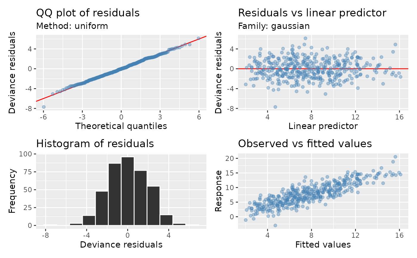
Model diagnostic plots

Model diagnostic plots

Usage

appraise(model, ...)

# S3 method for class 'gam'
appraise(
  model,
  method = c("uniform", "simulate", "normal", "direct"),
  use_worm = FALSE,
  n_uniform = 10,
  n_simulate = 50,
  seed = NULL,
  type = c("deviance", "pearson", "response"),
  n_bins = c("sturges", "scott", "fd"),
  ncol = NULL,
  nrow = NULL,
  guides = "keep",
  level = 0.9,
  ci_col = "black",
  ci_alpha = 0.2,
  point_col = "black",
  point_alpha = 1,
  line_col = "red",
  ...
)

# S3 method for class 'lm'
appraise(model, ...)

Arguments

model

a fitted model. Currently models inheriting from class "gam", as well as classes "glm" and "lm" from calls to stats::glm or stats::lm are supported.

...

arguments passed to patchwork::wrap_plots().

method

character; method used to generate theoretical quantiles. The default is "uniform", which generates reference quantiles using random draws from a uniform distribution and the inverse cumulative distribution function (CDF) of the fitted values. The reference quantiles are averaged over n_uniform draws. "simulate" generates reference quantiles by simulating new response data from the model at the observed values of the covariates, which are then residualised to generate reference quantiles, using n_simulate simulated data sets. "normal" generates reference quantiles using the standard normal distribution. "uniform" is more computationally efficient, but "simulate" allows reference bands to be drawn on the QQ-plot. "normal" should be avoided but is used as a fall back if a random number generator ("simulate") or the inverse of the CDF ("uniform"``) are not available from the family` used during model fitting.

Note that method = "direct" is deprecated in favour of method = "uniform".

use_worm

logical; should a worm plot be drawn in place of the QQ plot?

n_uniform

numeric; number of times to randomize uniform quantiles in the direct computation method (method = "direct") for QQ plots.

n_simulate

numeric; number of data sets to simulate from the estimated model when using the simulation method (method = "simulate") for QQ plots.

seed

numeric; the random number seed to use for method = "simulate" and method = "uniform".

type

character; type of residuals to use. Only "deviance", "response", and "pearson" residuals are allowed.

n_bins

character or numeric; either the number of bins or a string indicating how to calculate the number of bins.

ncol, nrow

numeric; the numbers of rows and columns over which to spread the plots.

guides

character; one of "keep" (the default), "collect", or "auto". Passed to patchwork::plot_layout()

level

numeric; the coverage level for QQ plot reference intervals. Must be strictly 0 < level < 1. Only used with method = "simulate".

ci_alpha, ci_col

colour and transparency used to draw the QQ plot reference interval when method = "simulate".

point_col, point_alpha

colour and transparency used to draw points in the plots. See graphics::par() section Color Specification. This is passed to the individual plotting functions, and therefore affects the points of all plots.

line_col

colour specification for the 1:1 line in the QQ plot and the reference line in the residuals vs linear predictor plot.

Note

The wording used in mgcv::qq.gam() uses direct in reference to the simulated residuals method (method = "simulated"). To avoid confusion, method = "direct" is deprecated in favour of method = "uniform".

See also

The plots are produced by functions qq_plot(), residuals_linpred_plot(), residuals_hist_plot(), and observed_fitted_plot().

Examples

load_mgcv()
## simulate some data...
dat <- data_sim("eg1", n = 400, dist = "normal", scale = 2, seed = 2)
mod <- gam(y ~ s(x0) + s(x1) + s(x2) + s(x3), data = dat)
## run some basic model checks
appraise(mod, point_col = "steelblue", point_alpha = 0.4)


## To change the theme for all panels use the & operator, for example to
## change the ggplot theme for all panels
library("ggplot2")
if (packageVersion("ggplot2") <= "3.5.2") {
  # Throws warning with ggplot rc 4.0.0 and patchwork 1.3.1 - will be fixed
  # in patchwork 1.3.2 - so temporarily skipping during ggplot release
  # process
  appraise(mod, seed = 42,
    point_col = "steelblue", point_alpha = 0.4,
    line_col = "black"
  ) & theme_minimal()
}