Simultaneous bands on an evaluation grid or a continuous interval

Simulation calibrates Gaussian bands jointly over the returned evaluation points. Tube calibration covers a continuous interval for supported one-dimensional cubic splines, including the space between returned points.

Details

Request interval = "simultaneous" and simultaneous_method = "tube". The simulation method remains the default. Tube bands use the same Gaussian coefficient covariance selected by frequentist and unconditional as simulation. For smooth estimates they also retain overall_uncertainty. They calibrate separately for each smooth or factor-level comparison; they do not cover all comparisons jointly.

Let $d(x)$ be the uncertainty design and $V$ the coefficient covariance. With $V=LL^T$, set $u(x)=L^Td(x)/\sqrt{d(x)^TVd(x)}$. The method integrates $\kappa=\int_a^b\|u'(x)\|\,dx$ and chooses $c$ so that $$2\{1-\Phi(c)\}+\kappa\exp(-c^2/2)/\pi=1-\mathrm{level}.$$ This expression bounds the two-sided exceedance probability by counting threshold crossings of the standardized Gaussian process. Repeated paths can make it conservative. Regular components separated by zero variance receive separate endpoint contributions. Polynomial knots divide numerical integration, but do not add endpoint contributions when the process is continuous. Zero-variance and rank-one processes are handled separately.

Under the selected Gaussian approximation, the band has at least the requested simultaneous probability over the stated interval, subject to numerical accuracy. Bayesian covariance gives an approximate posterior interpretation. Frequentist covariance calibrates centered Gaussian sampling errors; coverage of an unknown fixed curve also depends on smoothing bias. The unconditional covariance correction retains its existing meaning and does not integrate the full smoothing-parameter posterior. Numerical integration error estimates are diagnostics, not certified error bounds.

Supported quantities

Ordinary one-dimensional cubic regression splines ("cr", "cs"), cubic P-splines ("ps" with their ordinary cubic degree), and ordinary cubic thin plate bases ("tp", "ts") are supported. Factor-by smooths define separate curves. Numeric by multipliers must be fixed throughout each curve. Unconstrained GAMs and their BAM, GAMM, and GAMM4 adapters use their fitted prediction basis and covariance. Surfaces, constrained models, shape enforcement, and unsupported bases produce an error; there is no automatic switch to simulation.

First and second derivative bands retain the requested finite-difference functional, stencil, and step. The operator is evaluated using integrals of spline derivatives to avoid subtracting nearly equal basis values. This can improve floating-point accuracy relative to the simulation path without changing the mathematical functional. The continuous band refers to that derivative approximation. Differentiation must be on the smooth coordinate (wrt = "smooth", or the same coordinate on the covariate scale). Raw-scale derivatives of transformed terms are not supported by tube calibration. Difference bands retain the joint covariance of the two smooths and include group means when requested. The selected parametric group contributions must be constant along the curve.

Domain and numerical controls

simultaneous_domain accepts two increasing finite endpoints, or a named list keyed by coordinate. By default it is the range of returned evaluation coordinates, including gaps. A single evaluation location requires an explicit interval. All returned points must lie inside the domain, which must lie inside the fitted spline support; derivative stencils must also remain inside that support. The domain does not imply that each compared group has observations throughout it. With a fixed domain, n changes output density but does not change calibration. Connecting plotted bounds by straight segments is a rendering approximation to the continuous band.

tube_control accepts rel_tol = 1e-6, abs_tol = 1e-8, subdivisions = 1000L, and root_tol = 1e-8. Integration is split at polynomial boundaries and checked for convergence. Failures produce errors. Simulation controls (n_sim, n_cores/ncores, and seed) are ignored; tube calibration does not use random numbers. Computation controls require the fitted model. Drawing saved estimates uses their stored interval limits.

Returned metadata

The interval_info attribute records calibration = "tube", calculation = "tube_crossing_bound", the Gaussian covariance flags, and the per-smooth or per-comparison coverage scope. Its curves list contains identities, coordinates, resolved domains and their sources, critical values, lengths, regular-component counts, numerical diagnostics, and derivative stencils and steps where applicable. Methodological details are not added to plot captions.

References

Sun, J. and Loader, C. R. (1994). Simultaneous confidence bands for linear regression and smoothing. The Annals of Statistics, 22, 1328–1345. doi:10.1214/aos/1176325631 .

Krivobokova, T., Kneib, T. and Claeskens, G. (2010). Simultaneous confidence bands for penalized spline estimators. Journal of the American Statistical Association, 105, 852–863. doi:10.1198/jasa.2010.tm09165 .

Wiesenfarth, M., Krivobokova, T., Klasen, S. and Sperlich, S. (2012). Direct simultaneous inference in additive models and its application to model undernutrition. Journal of the American Statistical Association, 107, 1286–1296.

Liebl, D. and Reimherr, M. (2023). Fast and fair simultaneous confidence bands for functional parameters. Journal of the Royal Statistical Society: Series B, 85, 842–868. doi:10.1093/jrsssb/qkad026 .

Examples

library("mgcv")
set.seed(4)
dat <- data.frame(x = seq(0, 1, length.out = 100))
dat$y <- sin(6 * dat$x) + rnorm(100, sd = 0.2)
model <- gam(y ~ s(x, bs = "cr", k = 8), data = dat, method = "REML")
band <- smooth_estimates(model,
  interval = "simultaneous",
  simultaneous_method = "tube", simultaneous_domain = c(0, 1)
)
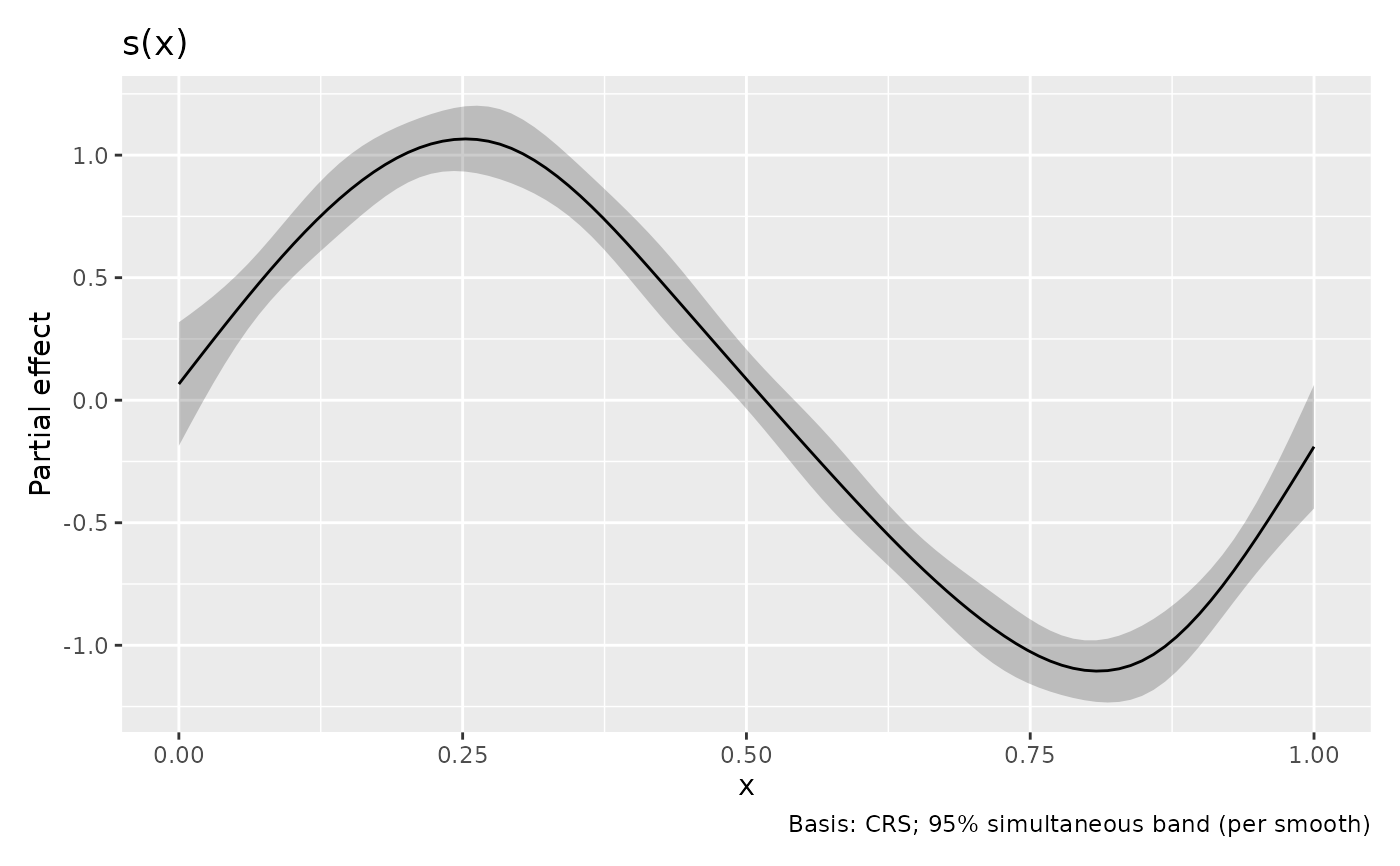
draw(band)

rate <- derivatives(model,
  type = "central", interval = "simultaneous",
  simultaneous_method = "tube"
)
attr(rate, "interval_info")$curves[[1]]$critical
#> [1] 3.015127