Formula effects for sdmTMB models

Evaluate and plot formula smooths and parametric effects from a fitted sdmTMB model using the same plotting methods as mgcv smooths. Penalized and unpenalized coefficients and their joint covariance are transformed back to the constrained mgcv basis.

Usage

# S3 method for class 'sdmTMB'
smooths(object, ...)

# S3 method for class 'sdmTMB'
n_smooths(object)

# S3 method for class 'sdmTMB'
get_smooths_by_id(object, id, ...)

# S3 method for class 'sdmTMB'
smooth_coefs(object, select, ...)

# S3 method for class 'sdmTMB'
smooth_estimates(
  object,
  ...,
  unconditional = FALSE,
  frequentist = FALSE,
  envir = NULL
)

# S3 method for class 'sdmTMB'
parametric_terms(model, ...)

# S3 method for class 'sdmTMB'
parametric_effects(
  object,
  terms = NULL,
  ...,
  unconditional = FALSE,
  frequentist = FALSE,
  envir = NULL
)

# S3 method for class 'sdmTMB'
assemble(
  object,
  ...,
  parametric = NULL,
  residuals = FALSE,
  unconditional = FALSE,
  frequentist = FALSE,
  envir = NULL,
  time_varying_style = c("ribbon", "pointrange")
)

# S3 method for class 'sdmTMB'
draw(
  object,
  ...,
  parametric = NULL,
  residuals = FALSE,
  unconditional = FALSE,
  frequentist = FALSE,
  envir = NULL,
  time_varying_style = c("ribbon", "pointrange")
)

Arguments

object, model

A fitted sdmTMB model.

...

Arguments passed to the corresponding gratia methods, including grid, interval, transformation, surface, styling and layout controls. For threshold terms, n sets the number of evenly spaced evaluation points over the fitted covariate range; a fitted breakpoint within that range is also included. Supplied data determines evaluation locations.

id

Integer positions of smooths across model components.

select

Smooth selection across both predictors of delta models. Numeric and logical indices follow stored smooth order, first component then second. Character selections use smooths() labels, such as s(x) and s.1(x) for the second component.

unconditional, frequentist

Must be FALSE. Intervals use the joint RTMB covariance; mgcv-specific alternatives are unavailable.

envir

Optional environment for evaluating model covariates.

terms

Parametric terms to evaluate or draw, as returned by parametric_terms(), including breakpt(x) and logistic(x) threshold terms and time_varying(temperature) coefficient trajectories. Second-component selectors have a .1 suffix.

parametric

Include parametric effects? NULL includes them unless smooths are selected explicitly, as for draw.gam().

residuals

Must be FALSE; partial residuals are not supported.

time_varying_style

Display time-varying coefficients with a line, points and uncertainty ribbon ("ribbon", the default), or with points, interval bars and a faint connecting line ("pointrange").

Value

Smooth labels, smooth objects, coefficients, effect estimates, or plots, as for the corresponding GAM methods. draw() returns a patchwork, or named panels with wrap = FALSE; assemble() returns an assembled_plots list. Models without smooths can draw parametric effects.

Details

Use smooths() to list smooth names, get_smooth() to extract an exact name, get_smooths_by_id() to extract by position, and n_smooths() to count smooths, including both predictors of a delta model. These utilities do not calculate coefficient covariances.

Smooth, ordinary parametric and threshold estimates are partial contributions on each component's link scale. Spatial, spatiotemporal, IID random effects, offsets and varying coefficients are not added to these effects. Their influence on coefficient uncertainty is retained through the joint covariance. Smooth intervals include uncertainty in their component's overall mean by default; parametric intervals include the component's intercept. Use overall_uncertainty = FALSE for term-only intervals. fun transforms displayed partial effects, not full predictions. Use surface = "3d", ci_3d = TRUE in draw() or assemble() to add interval surfaces to smooths and numeric parametric interactions in either component. ci_3d_alpha and ci_3d_col control their opacity and fill colour. Pass cyclic = "polar" and optional polar_args to draw() or assemble() for polar plots of supported one-dimensional cyclic smooths. See draw.gam() for the coordinate options.

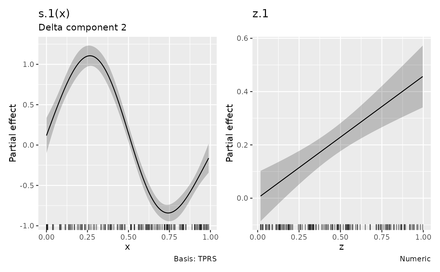
Delta components have separate smooth and parametric coefficients and are drawn separately, with component subtitles. Upstream sdmTMB restrictions on supported bases and delta formulas still apply. Tensor smooths with multiple penalties are supported. Fits require stored smooth metadata; mapping or profiling required coefficients and non-positive-definite Hessians give errors. Parametric subtitles also identify the component for threshold curves and time-varying coefficients. Saved parametric_effects() retain the labels in an optional .model column.

Support requires sdmTMB >= 1.2.0 models fitted with the RTMB backend. Refit older models or TMB fits with control = sdmTMB::sdmTMBcontrol(backend = "rtmb"). Diagnostics use complete fitted predictors, including spatial, spatiotemporal and independent group effects and offsets. Supported single-response and standard delta families provide PIT/quantile residuals, ordinary and scalable diagnostic plots, and joint approximate posterior predictive checks. Delta diagnostics can select the complete response, occurrence or positive component. Raw posterior response draws are available through posterior_samples(). By default, fields are drawn together once from their approximate posterior and held fixed (mle-mvn), following sdmTMB's recommended residual calculation. Checks can also hold estimates fixed, average over fitted-field uncertainty, or simulate new fields. Marginal simulations preserve dependence and supply residual ranks, including for nonlinear and coupled delta responses. See diagnostic_support for treatment of coefficients, fields and covariance, and what each check assesses.

Threshold curves are partial contributions without centring. They follow parametric selection rules: terms selects them and parametric = FALSE excludes them. Both delta components have separate threshold parameters. Threshold intervals use the delta method with the joint covariance of the fitted parameters, including uncertainty in the breakpoint or logistic width. By default they include intercept uncertainty and its covariance with the curve, without adding the intercept to the estimated contribution. Use overall_uncertainty = FALSE for term-only uncertainty. At the breakpoint, the derivative is taken from the constant side, matching native sdmTMB prediction. Threshold intervals remain pointwise when simultaneous smooth bands are requested. Rugs show fitting observations.

Time-varying coefficients are plotted at their stored time steps, including extra_time; n does not add time steps. Select each fitted design column with a label such as time_varying(temperature) or time_varying(Intercept). A covariate named Intercept is distinguished from the intercept by backticks: time_varying(`Intercept`). Factor contrasts, transformations and interactions retain the fitted coefficient coding. For rw, estimates are the temporal coefficients. For rw0 and ar1, the matching ordinary coefficient is added to its temporal deviation. Their joint covariance includes the variance of both parts and their covariance. An absent ordinary coefficient contributes zero. Matching columns must have compatible coding in the main and temporal designs. Default effects omit ordinary terms whose coefficients are already included in trajectories; their ordinary selectors remain available for explicit requests. overall_uncertainty governs ordinary partial effects; temporal panels always retain their complete coefficient covariance. Temporal intervals remain pointwise when simultaneous smooth bands are requested. Supplied data selects stored time steps if it contains the model's time column; otherwise all stored times are retained. Missing or unknown requested times give an error. sdmTMB 1.2.0 requires numeric time values for time-varying processes.

Time-varying estimates from parametric_effects() use .type = "time_varying", .value for time, .partial for the full coefficient, and .se for its standard error. Both display styles are also available through draw.parametric_effects(), including nested saved estimates.

Smooth extraction and effect plots do not support dispersion formulas, other multi-predictor families, or nonlocal effects. Spatial fields and group random effects are not plotted.

Label layout

Pass label_control = draw_label_control(...) to draw() to wrap discrete axis labels and legend text, stagger discrete tick labels, or adjust legend and colour-bar layout. Settings apply to each panel, including unwrapped plot lists. See draw_label_control() for the available settings.

Examples

if (requireNamespace("sdmTMB", quietly = TRUE)) {
  load_mgcv()
  # Simulate nonlinear and linear effects with Gaussian noise
  set.seed(42)
  d <- data.frame(x = runif(150), z = runif(150))
  d$y <- 1 + sin(6 * d$x) + 0.5 * d$z + rnorm(150, sd = 0.3)

  # Fit without a spatial field and draw the linear and smooth effects
  m <- sdmTMB::sdmTMB(y ~ z + s(x, k = 6), data = d, spatial = "off")
  smooths(m)
  draw(m)
}