Extend diagnostics for an mgcv-compatible family

A family can supply a gratia_diagnostics function to describe its response distribution without adding family-name checks to gratia. The function is called with named arguments mu, wt, scale, y and eta. These contain response parameters, weights, fitted scale, the fitting response and linear predictors, respectively. Diagnostics use fitted parameters and sampling weights; log_lik() uses draw-specific parameters and likelihood weights. Missing fitting rows have been removed; grouped families receive only their own rows. eta can be NULL when a distribution is constructed without a fitted model.

Details

Return a named list. Omitted fields retain gratia's existing family defaults; an explicit NULL removes an optional function or moment. Existing $rd, $cdf and $qf functions are preserved and supplied with their usual mgcv arguments. Replacement functions in the returned list instead capture fitted parameters and use the following interface:

mean, variance: numeric response moments, one per observation. A matrix is allowed for multiple response columns. Use the full response expectation, rather than a location parameter or a component mean.
cdf, cdf_left: functions (q, log_p = FALSE, lower_tail = TRUE) for P(Y <= q) and P(Y < q), respectively. They must support both tails and logarithms. For an upper tail, cdf_left returns P(Y >= q).
qf: a function (p, log_p = FALSE, lower_tail = TRUE) for quantiles.
rd: a function with no arguments that draws a complete response vector (or response matrix), retaining any dependence between observations.
log_lik: a function (y) returning one normalised log density or log probability mass per observation, including fitting weights. A response vector contributes one value; a multivariate response contributes one joint value per row. log_lik() calls the factory at each coefficient draw with likelihood weights, which can differ from diagnostic sampling weights. Parameters represented by mu and eta vary with that draw; the hook must exclude smoothing penalties and priors. Finite positive log densities and -Inf for impossible observations are allowed; missing values and Inf are invalid.
bounds: a function (y) returning a list with numeric lower and upper response bounds. Censoring intervals use their endpoints. Exact count observations can use y - 1 and y. Alternatively, supply cdf_left: gratia then randomises between P(Y < y) and P(Y <= y) automatically. A bounds list may also supply cdf_lower and cdf_upper, functions (log_p = FALSE, lower_tail = TRUE) that evaluate its endpoint probabilities, and left_limit, a logical vector marking rows to randomise at equal bounds.
continuous: set to TRUE to declare that responses have no probability masses. An unfamiliar grouped-family component must supply bounds, cdf_left, or this declaration before using PIT/quantile residuals.
diagnostic_residuals: a function (y, type) for observed and reference deviance, response and Pearson residuals. Otherwise the family's existing residual method is used.
observe: a function (y) applying an observation process, such as known censoring thresholds, to generated responses before traditional QQ/worm reference residuals are calculated. Return the response encoding expected by the family's residual method. This function is not applied to fitting observations or to the public response and posterior samplers.
reference_available, reference_reason: a single logical value and an explanation. Set availability to FALSE when traditional distribution-based references cannot be generated, for example when censoring thresholds are unknown. Analytic PIT/quantile plots remain available.
mean_available, variance_available, moment_reason: single logical values specifying whether the population moments exist, and an explanation used when a requested residual requires an undefined moment.
independent, joint_available, dependence_reason: single logical values describing independence and availability of joint response draws, and an explanation of dependence. joint_available requires an rd function.
approximation: an optional explanation shown in diagnostic subtitles.

Functions must return one value per response in fitting order. Probabilities must be valid and lower bounds must not exceed upper bounds. gratia validates supplied values and reports errors instead of silently using another method. The factory is called again for each prepared distribution; avoid changing the family or drawing random numbers in the factory itself.

Adding this function does not extend a family's supported fitting methods. Posterior predictive sampling still uses the fitting package's parameter and response sampling methods. The likelihood hook also operates at supplied coefficient draws.

Examples

load_mgcv()
f <- poisson()
f$gratia_diagnostics <- function(mu, wt, scale, y, eta) {
  list(mean = mu, variance = mu,
    cdf_left = function(q, log_p = FALSE, lower_tail = TRUE) {
      ppois(ceiling(q) - 1, lambda = mu,
        log.p = log_p, lower.tail = lower_tail)
    })
}
dat <- data.frame(x = seq(0, 1, length.out = 40))
dat$y <- rep(c(0, 1, 2, 4), 10)
f$rd <- function(mu, wt, scale) rpois(length(mu), mu)
f$qf <- function(p, mu, wt, scale) qpois(p, mu)
f$cdf <- function(q, mu, wt, scale) ppois(q, mu)
fit <- gam(y ~ x, data = dat, family = f, method = "REML")
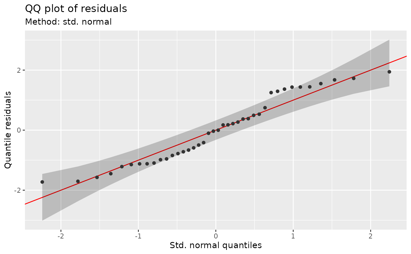
qq_plot(fit, type = "quantile", seed = 1)

Details

See also

Examples