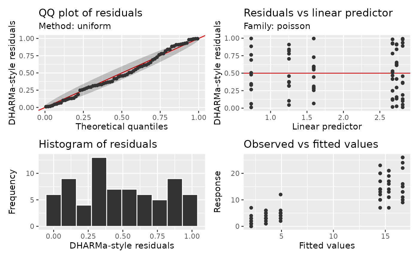
Calculate DHARMa-style residuals using gratia's fitted response generators. No DHARMa or mgcViz installation is needed.
Arguments
- model
a fitted model supported by diagnostic_support, with a generator for comparable scalar responses.
- n
positive integer; number of response datasets to simulate.
- seed
integer or
NULL; random seed for randomised residuals. WithNULL, calculations use the current random-number state. An explicit seed preserves the caller's state, including when none was previously initialised.- conditioning
character or
NULL; hold fitted random effects fixed ("conditional"), average over new effects ("marginal"), or use the extracted GAM ("gam_component"), where supported. See diagnostic_support.- ...
model-specific diagnostic options, including sdmTMB's
componentandfield_method.
Value
A numeric vector in observation order. With na.exclude, excluded
observations are restored as NA; with na.omit, only fitting rows remain.
Details
For each observation, calculate the fractions of simulated responses strictly below it and below or equal to it. The residual is sampled uniformly between these fractions when simulations tie with the observation. Without ties it is the fraction strictly below the observation. This implements DHARMa's PIT idea internally, using gratia's response distributions and conditioning rules.
Residuals lie in [0, 1]. An observation below every simulated response has
residual zero; one above every simulated response has residual one. Endpoints
are retained. Increasing n improves the resolution of the empirical CDF.
Continuous responses without ties have residuals on the grid 0:n / n.
Responses are generated together to retain any modelled dependence. When only marginal response draws are available, these residuals describe the marginal distributions. Censored observations and multivariate responses are unsupported. Binomial successes and failures are compared as proportions with the model's fitting trial counts. A response CDF and finite response moments are not required.
Use type = "dharma" and n_dharma in diagnostic plots. QQ and worm plots
use uniform reference quantiles. Independent responses have approximate
pointwise order-statistic bands: the finite simulation grid means the
continuous uniform reference is approximate. Bands are omitted for dependent
responses because independence-based intervals do not describe their order
statistics. These checks use fitted parameters without refitting the model.
An explicit seed preserves the caller's random-number state. With
seed = NULL, simulation and tie randomisation advance the current state.
References
Hartig, F. DHARMa: Residual Diagnostics for Hierarchical (Multi-Level / Mixed) Regression Models. doi:10.32614/CRAN.package.DHARMa .