Plot smooth and parametric terms from a fitted GAM

Plots smooth and parametric contributions from a fitted GAM model using ggplot2::ggplot().

Usage

# S3 method for class 'gam'
assemble(
  object,
  data = NULL,
  select = NULL,
  parametric = NULL,
  terms = NULL,
  residuals = FALSE,
  scales = c("free", "fixed"),
  ci_level = 0.95,
  n = 100,
  n_2d = 50,
  n_3d = 16,
  n_4d = 4,
  unconditional = FALSE,
  overall_uncertainty = TRUE,
  constant = NULL,
  fun = NULL,
  dist = 0.1,
  rug = TRUE,
  distinct_rug = TRUE,
  contour = TRUE,
  grouped_by = FALSE,
  ci_alpha = 0.2,
  ci_col = "black",
  smooth_col = "black",
  resid_col = "steelblue3",
  contour_col = "black",
  n_contour = NULL,
  partial_match = FALSE,
  discrete_colour = NULL,
  discrete_fill = NULL,
  continuous_colour = NULL,
  continuous_fill = NULL,
  position = "identity",
  angle = NULL,
  ncol = NULL,
  nrow = NULL,
  guides = "keep",
  widths = NULL,
  heights = NULL,
  crs = NULL,
  default_crs = NULL,
  lims_method = "geometry_bbox",
  wrap = TRUE,
  caption = TRUE,
  envir = NULL,
  surface = c("raster", "tile", "3d"),
  surface_3d = list(),
  ci_3d = FALSE,
  ci_3d_alpha = 0.15,
  ci_3d_col = "grey60",
  back_transform = FALSE,
  re_levels = NULL,
  mrf_plot = c("effects", "qq"),
  interval = c("confidence", "simultaneous"),
  n_sim = 10000,
  n_cores = 1,
  seed = NULL,
  interval_method = c("auto", "gaussian", "bootstrap", "shape"),
  frequentist = FALSE,
  shape_source = c("gaussian", "bootstrap"),
  ...,
  variables = NULL,
  simultaneous_method = c("simulation", "tube"),
  simultaneous_domain = NULL,
  tube_control = list()
)

# S3 method for class 'scam'
assemble(object, ..., overall_uncertainty = FALSE, centre = c("model", "plot"))

Arguments

object

a fitted GAM, the result of a call to mgcv::gam().

data

an optional data frame that is used to supply the data at which the smooths will be evaluated and plotted. This is usually not needed, but is an option if you need fine control over exactly what data are used for plotting.

select

character, logical, or numeric; which smooths to plot. If NULL, the default, then all model smooths are drawn. Numeric select indexes the smooths in the order they are specified in the formula and stored in object. Character select matches the labels for smooths as shown for example in the output from summary(object). Logical select operates as per numeric select in the order that smooths are stored.

parametric

logical or NULL; plot parametric terms also? The default, NULL, includes parametric terms when select = NULL, but excludes them when smooths are selected explicitly. Use TRUE to include parametric terms regardless of select, or FALSE to draw only smooths (the previous default). The terms argument selects which parametric effects are plotted; select selects only smooths.

terms

character; which model parametric terms should be drawn? The Default of NULL will plot all parametric terms that can be drawn. Interactions show their individual contributions to the linear predictor; main effects and intercepts are not added. Multivariate parametric terms use the grid and surface controls below, as described in parametric_effects().

residuals

logical; should partial residuals for a smooth be drawn? Ignored for anything but a simple univariate smooth. If the model does not provide working residuals and working weights, warns once and draws the smooths without partial residuals.

scales

character; should all univariate smooths be plotted with the same y-axis scale? If scales = "free", the default, each univariate smooth has its own y-axis scale. If scales = "fixed", a common y axis scale is used for all univariate smooths.

Currently does not affect the y-axis scale of plots of the parametric terms.

ci_level

numeric between 0 and 1; the coverage of credible interval.

n

numeric; the number of points over the range of the covariate at which to evaluate a univariate smooth.

n_2d

numeric; the number of points along each of the first two axes of a smooth surface, including surface panels of higher-dimensional smooths. The default is 50 in plotting and plot-preparation functions. If NULL, use n instead. Ignored when evaluation data are supplied. Factor levels are retained, and curves with only one continuous covariate use n.

n_3d

numeric; the number of new observations to generate for the third dimension of a 3D smooth. Factor conditioning dimensions retain at most this many levels, taking the first levels in fitted order. Explicit re_levels selections take precedence; supplied data are unchanged.

n_4d

numeric; the number of new observations to generate for the dimensions higher than 2 (!) of a kD smooth (k >= 4). For example, if the smooth is a 4D smooth, each of dimensions 3 and 4 will get n_4d new observations. For factor conditioning dimensions, this is the maximum number of levels retained per dimension, taking the first in fitted order. Explicit re_levels selections take precedence; supplied data are unchanged.

unconditional

logical; should confidence intervals include the uncertainty due to smoothness selection? If TRUE, the corrected Bayesian covariance matrix will be used.

overall_uncertainty

logical; should the uncertainty in the model constant term be included in the standard errors of smooth and parametric effects? For parametric effects this includes the intercept variance and its covariance with the term, without changing the partial estimates. Each term uses the intercept of its own linear predictor. Native scasm models are routed to draw.scasm() with overall_uncertainty = FALSE. An explicit request for unavailable mean uncertainty warns once. The stored model class is unchanged.

constant

numeric; a constant to add to the estimated values of the smooth. constant, if supplied, will be added to the estimated value before the confidence band is computed.

fun

function; a function that will be applied to the estimated values and confidence interval before plotting. Can be a function or the name of a function. For simultaneous bands it must be monotone over the entire band; endpoint transformation alone does not preserve non-monotone band coverage. Function fun will be applied after adding any constant, if provided.

dist

numeric; if greater than 0, this is used to determine when a location is too far from data to be plotted when plotting 2-D smooths. The data are scaled into the unit square before deciding what to exclude, and dist is a distance within the unit square. See mgcv::exclude.too.far() for further details.

rug

logical; draw a rug plot at the bottom of each plot for 1-D smooths or plot locations of data for higher dimensions.

distinct_rug

logical; should the data for the rug plots be reduced to the distinct values?

contour

logical; should contours be draw on the plot using ggplot2::geom_contour().

grouped_by

logical; should factor by smooths be drawn as one panel per level of the factor (FALSE, the default), or should the individual smooths be combined into a single panel containing all levels (TRUE)?

ci_alpha

Deprecated; use gratia_theme_get() theme settings instead. Numeric; alpha transparency for confidence or simultaneous interval.

ci_col

Deprecated; use gratia_theme_get() theme settings instead. Colour specification for the confidence/credible intervals band. Affects the fill of the interval.

smooth_col

Deprecated; use gratia_theme_get() theme settings instead. Colour specification for the smooth line.

resid_col

Deprecated; use gratia_theme_get() theme settings instead. Colour specification for the partial residuals.

contour_col

Deprecated; use gratia_theme_get() theme settings instead. Colour specification for contour lines.

n_contour

numeric; the number of contour bins. Will result in n_contour - 1 contour lines being drawn. See ggplot2::geom_contour().

partial_match

logical; should smooths be selected by partial matches with select? If TRUE, select can only be a single string to match against.

discrete_colour

a suitable colour scale to be used when plotting discrete variables.

discrete_fill

a suitable fill scale to be used when plotting discrete variables.

continuous_colour

a suitable colour scale to be used when plotting continuous variables.

continuous_fill

a suitable fill scale to be used when plotting continuous variables.

position

Position adjustment, either as a string, or the result of a call to a position adjustment function.

angle

numeric; the angle at which the x axis tick labels are to be drawn passed to the angle argument of ggplot2::guide_axis().

ncol, nrow

numeric; the numbers of rows and columns over which to spread the plots

guides

character; one of "keep" (the default), "collect", or "auto". Passed to patchwork::plot_layout()

widths, heights

The relative widths and heights of each column and row in the grid. Will get repeated to match the dimensions of the grid. If there is more than 1 plot and widths = NULL, the value of widths will be set internally to widths = 1 to accommodate plots of smooths that use a fixed aspect ratio.

crs

the coordinate reference system (CRS) to use for the plot. All data will be projected into this CRS. See ggplot2::coord_sf() for details.

default_crs

the coordinate reference system (CRS) to use for non-sf layers added to spherical plots. The default, NULL, uses 4326 (WGS84). Internally generated surface cells, contours and observation points have their own geographic CRS, with longitude on the horizontal axis and latitude on the vertical axis. See ggplot2::coord_sf() for more details.

lims_method

character; affects how spherical plot axis limits are determined. The default, "geometry_bbox", uses the rendered geometry. Passed to ggplot2::coord_sf(). Spherical surfaces use explicit geographic cells with valid polar and date-line boundaries. Orthographic plots clip cells, contours and observation points to the visible hemisphere before projection. Explicit prediction data on a rectilinear grid retain their actual spacing; scattered or singleton coordinates are drawn as points, with a message, because they do not define surface cells. Incomplete observation rug coordinates are omitted. Grouped factor-by spherical surfaces use separate facets for each factor level.

wrap

logical; wrap plots as a patchwork? If FALSE, a list of ggplot objects is returned, 1 per term plotted.

caption

logical; show the smooth type in the caption of each plot?

envir

an optional environment for looking up data, functions and constants. Defaults to the model's evaluation environment.

surface

character; one of "raster" (the default), "tile", or "3d". Raster surfaces keep large PDF plots compact; tiles are borderless vector rectangles. Three-dimensional surfaces use the optional ggcube package, with the displayed partial effect as height and fill. Numeric smooth and parametric surfaces, including conditioning facets and soap films, are supported. Curves and factor estimates keep their usual display; spherical smooths retain their geographic rendering. Covariate scale changes that produce irregular spacing use rectangles bounded by adjacent coordinate midpoints for flat surfaces.

surface_3d

named list of view options passed to ggcube::coord_3d(), for example list(yaw = 45, persp = FALSE). The default list() uses the default view with ggcube::light(backface_scale = 1), preserving equal horizontal units for isotropic smooths. Supply light = ggcube::light(...) in this list to override lighting; ggcube::light(method = "none") disables it. An explicitly supplied light replaces the entire default light. Only the coordinate system is used; ggcube's theme settings are not applied. These options affect all 3D panels in a call. For different views per term, modify individual plots returned by assemble(). The dist entry here controls perspective; the top-level dist argument controls masking.

ci_3d

logical; add lower and upper interval surfaces to numeric smooth and parametric effect panels when surface = "3d"? Defaults to FALSE. Applies across supported model classes and conditioning facets. Other panel types, including standard errors, retain their usual display. Smooth bounds follow interval; parametric bounds remain pointwise.

ci_3d_alpha

Deprecated; use gratia_theme_get() theme settings instead. Numeric between 0 and 1; opacity of both interval surfaces, independent of ci_alpha. Defaults to 0.15.

ci_3d_col

Deprecated; use gratia_theme_get() theme settings instead. One R colour; fill of both interval surfaces, independent of ci_col and the estimate's continuous fill scale. Defaults to "grey60".

back_transform

logical; plot covariates on their original scale? Defaults to FALSE, using model coordinates such as log(x) for a term containing log(x). With TRUE, recover the raw covariates, generate a grid on their original scale and evaluate the model expressions forwards. Applies to axes, rugs, partial-residual locations and conditioning facets, including tensor products and parametric interactions. Each smooth axis must depend on one distinct original model covariate. Functions such as foo(x) are supported when their raw inputs and functions can be recovered; no inverse function is needed. Missing raw data or unavailable functions produce an error; supply data or envir as appropriate. With supplied prediction data, unavailable raw fitting observations omit rugs and partial residuals; prediction rows are never used as observations. For precomputed smooth estimates, prepare raw grids with smooth_estimates(model, back_transform = TRUE) before drawing with back_transform = TRUE. Raw inputs supplied through data also retain their coordinates. Transformed-only estimates cannot be relabelled on the raw scale, including grids carrying typical values from include_all = TRUE. Transformed soap-film boundaries lack retained raw coordinates and must be drawn with back_transform = FALSE. Parametric estimates retain both scales; multi-column basis expansions retain raw axes on either setting. Does not transform estimated effects or their intervals; use fun for that.

re_levels

named list of factor level labels to retain in tensor products with random-effect margins, for example list(species = c("a", "b")). Fitted factor order and ordered status are retained.

mrf_plot

character; display Markov random field smooths as area-labelled estimates and intervals ("effects", the default), or a descriptive Gaussian quantile plot ("qq"). MRF effects are correlated and need not have equal marginal variances; the QQ display is not a test of independent normal effects. Specialist maps and graph plots are outside the scope of this display.

interval

character; "confidence" (default) draws pointwise intervals; "simultaneous" uses a band across, by default, the finite evaluation grid of each smooth, including its slices and factor levels. Separate smooths are not a joint coverage set. "credible" aliases "confidence", reflecting the approximate Bayesian credible interpretation of default-covariance bands. Parametric panels retain pointwise intervals and are labelled accordingly when simultaneous smooth bands are requested. Bands appear where the renderer displays interval bounds, including 3D effect surfaces when ci_3d = TRUE. Random-effect QQ plots retain their usual display. simultaneous_method = "tube" calibrates supported univariate bands over a continuous interval; see simultaneous_bands.

n_sim, n_cores

positive integers; coefficient draws and simulation cores for simultaneous bands. Parallel simulation requires OpenMP support.

seed

integer or NULL; an explicit simulation seed preserves the caller's RNG state.

interval_method

character; "auto" uses stored scasm bootstrap draws for pointwise intervals when available, and Gaussian intervals otherwise. Use "gaussian" to request covariance-based limits or "bootstrap" to require stored draws. Simultaneous bootstrap bands are not supported. "shape" applies shape_intervals() to supported scasm smooth components, using the initial limits chosen by shape_source.

frequentist

logical; use frequentist covariance for smooth-component intervals? The default uses approximate Bayesian covariance. Parametric effect intervals retain their existing Bayesian covariance calculation.

shape_source

character; initial uncertainty for interval_method = "shape": "gaussian" (the default) or stored "bootstrap" pointwise limits. Bootstrap sources require frequentist = FALSE and unconditional = FALSE because the stored draws hold smoothing fixed.

...

Additional smooth plotting arguments, including title, subtitle, xlab and ylab.

variables

Character vector giving every covariate of the selected smooths exactly once, in plotting order: x, y, then the conditioning covariate for 3D smooths, or facet rows and columns for 4D smooths. When supplied, selected smooths must use the same covariates. Use fitted coordinate names, such as "log(x)" for a transformed covariate. The default, NULL, favours a two-variable tensor margin for x and y, otherwise retaining fitted order. Grid resolution follows this order. Supplied data are evaluated unchanged. Drawing saved estimates can change the order but uses only points already evaluated; evaluate again to change grid resolution or conditioning values. Continuous covariates must precede factors. Spherical smooths retain their latitude/longitude convention and do not support reordering.

simultaneous_method

character; calibration for simultaneous bands. The default, "simulation", uses coefficient draws on the evaluation grid. "tube" uses a conservative Gaussian threshold-crossing bound over a continuous interval for supported one-dimensional cubic splines. See simultaneous_bands.

simultaneous_domain

numeric pair of increasing finite endpoints, or a named list of such pairs keyed by spline coordinate. For tube bands, NULL uses the range of returned evaluation coordinates, including gaps. All returned points must lie inside the interval and the interval must lie inside the fitted spline support. Requires tube calibration.

tube_control

named list controlling numerical tube calibration: rel_tol (default 1e-6), abs_tol (1e-8), subdivisions (1000L), and root_tol (1e-8). Requires tube calibration. Simulation controls n_sim, n_cores (or ncores), and seed are ignored by tube calibration.

centre

character; for SCAM models, "model" retains each fitted smooth contribution. "plot" subtracts the evaluation-grid mean from each bivariate smooth to match scam::plot.scam(). The same linear transformation is applied to its covariance. Univariate curves and smooth_estimates() retain the fitted centring for either setting.

Value

A list of ggplot2::ggplot() objects.

Details

Smooth plot subtitles identify the model part or distributional parameter as described in draw.gam(). Custom smooth labels, including subtitle, can be passed through ....

Note

Internally, plots of each smooth are created using ggplot2::ggplot() and composed into a single plot using patchwork::wrap_plots(). As a result, it is not possible to use + to add to the plots in the way one might typically work with ggplot() plots. Instead, use the & operator; see the examples.

Author

Gavin L. Simpson

Examples

load_mgcv()

# simulate some data
df1 <- data_sim("eg1", n = 400, dist = "normal", scale = 2, seed = 2)
# fit GAM
m1 <- gam(y ~ s(x0) + s(x1) + s(x2) + s(x3), data = df1, method = "REML")

# assemble plots of all smooths
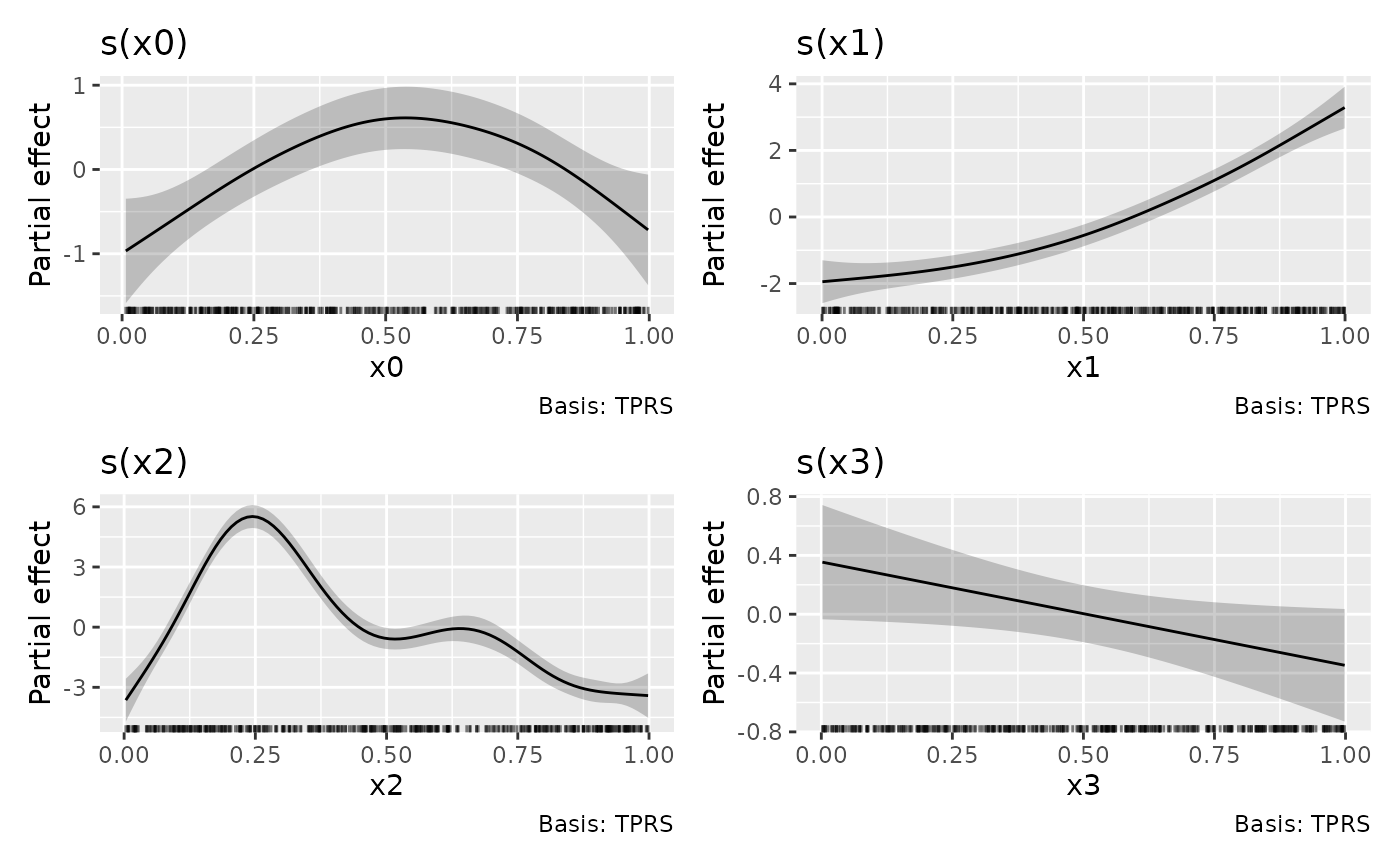
assemble(m1)
#> 
#> -- Assembly of 4 plots --
#> 
#> 1. s(x0)
#> 2. s(x1)
#> 3. s(x2)
#> 4. s(x3)
#> 

# can be passed to patchwork::wrap_plots()
suppressPackageStartupMessages(library("patchwork"))
assemble(m1) |> wrap_plots(ncol = 2, nrow = 2)