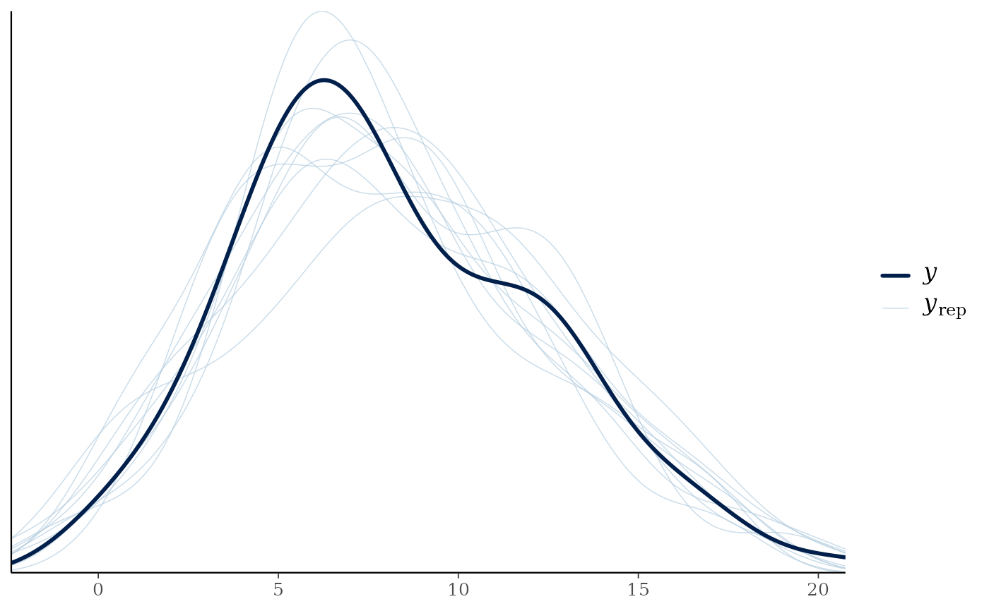
Compare observations with replicated responses using an optional installation
of bayesplot. Call bayesplot::pp_check() after loading gratia.
Usage
pp_check.gam(
  object,
  ...,
  type = "dens_overlay",
  prefix = c("ppc", "ppd"),
  n_draws = NULL,
  seed = NULL,
  group = NULL,
  x = NULL,
  response = NULL,
  conditioning = NULL,
  sampling_args = list()
)

pp_check.bam(
  object,
  ...,
  type = "dens_overlay",
  prefix = c("ppc", "ppd"),
  n_draws = NULL,
  seed = NULL,
  group = NULL,
  x = NULL,
  response = NULL,
  conditioning = NULL,
  sampling_args = list()
)

pp_check.gamm(
  object,
  ...,
  type = "dens_overlay",
  prefix = c("ppc", "ppd"),
  n_draws = NULL,
  seed = NULL,
  group = NULL,
  x = NULL,
  response = NULL,
  conditioning = NULL,
  sampling_args = list()
)

pp_check.gamm4(
  object,
  ...,
  type = "dens_overlay",
  prefix = c("ppc", "ppd"),
  n_draws = NULL,
  seed = NULL,
  group = NULL,
  x = NULL,
  response = NULL,
  conditioning = NULL,
  sampling_args = list()
)

pp_check.scam(object, ...)
Arguments
- object
a fitted GAM, BAM, gamm, or gamm4 model.
- ...
arguments passed only to the selected bayesplot plotting function.
- type
character; the bayesplot plot name without its
ppc_orppd_prefix. Available names come from the installed version of bayesplot.- prefix
character;
"ppc"compares responses with observations;"ppd"shows replicated responses alone.- n_draws
positive integer; total coefficient and response draws. Defaults to 50 for ordinary plots and 4000 for leave-one-out plots. With supplied coefficient draws, defaults to their number of rows.
- seed
integer or
NULL; seed for reproducible sampling.- group, x
a variable name in the fitting model frame, or a vector in fitting-row order. Missing fitting rows are removed with the response.
- response
character or integer; response column or grouped-family component to check, for example
"response2"or"component1". Required when the model contains several responses or grouped components.- conditioning
character or
NULL; conditioning passed to the existing posterior predictive sampler. Seeposterior_predictive_plot().- sampling_args
named list; arguments for the posterior sampler, including
method,draws,unconditional, andmvn_method. Prediction at new data is not supported. Fitted binomial trials must be retained. Usechainsfor multiple coefficient chains anddiagnostics = TRUEfor coefficient diagnostics. Leave-one-out plots use stored chain identities; for unlabelled supplied draws, includer_efforchain_idhere.
Details
These methods require bayesplot only when called. Leave-one-out plots also
require loo and a likelihood supported by log_lik(). Their response and
likelihood calculations use exactly the same coefficient draws. For a
multivariate response, the weights leave out the entire response vector.
Grouped-family checks use only the selected component's observations.
Some bayesplot plotting functions, including error_binned and LOO-PIT
plots, also require bayesplot's optional rstantools package. Install it with
install.packages("rstantools") to use those plots.
Binomial observations and replicated responses are shown as numbers of
successes with fitted trial counts. Other gratia predictive plots use
proportions. The error_binned plot uses expected responses rather than
response simulations and requires an available finite response mean. For
gamm and gamm4 it currently requires conditioning = "gam_component".
Plotting functions requiring additional inputs, such
as censoring indicators, receive those inputs through ....
Coefficient draws use a Gaussian approximation by default; additional family
parameters remain at fitted values. See log_lik() for the assumptions of
approximate leave-one-out calculations. Existing conditioning and response
dependence restrictions of the diagnostic samplers also apply here.