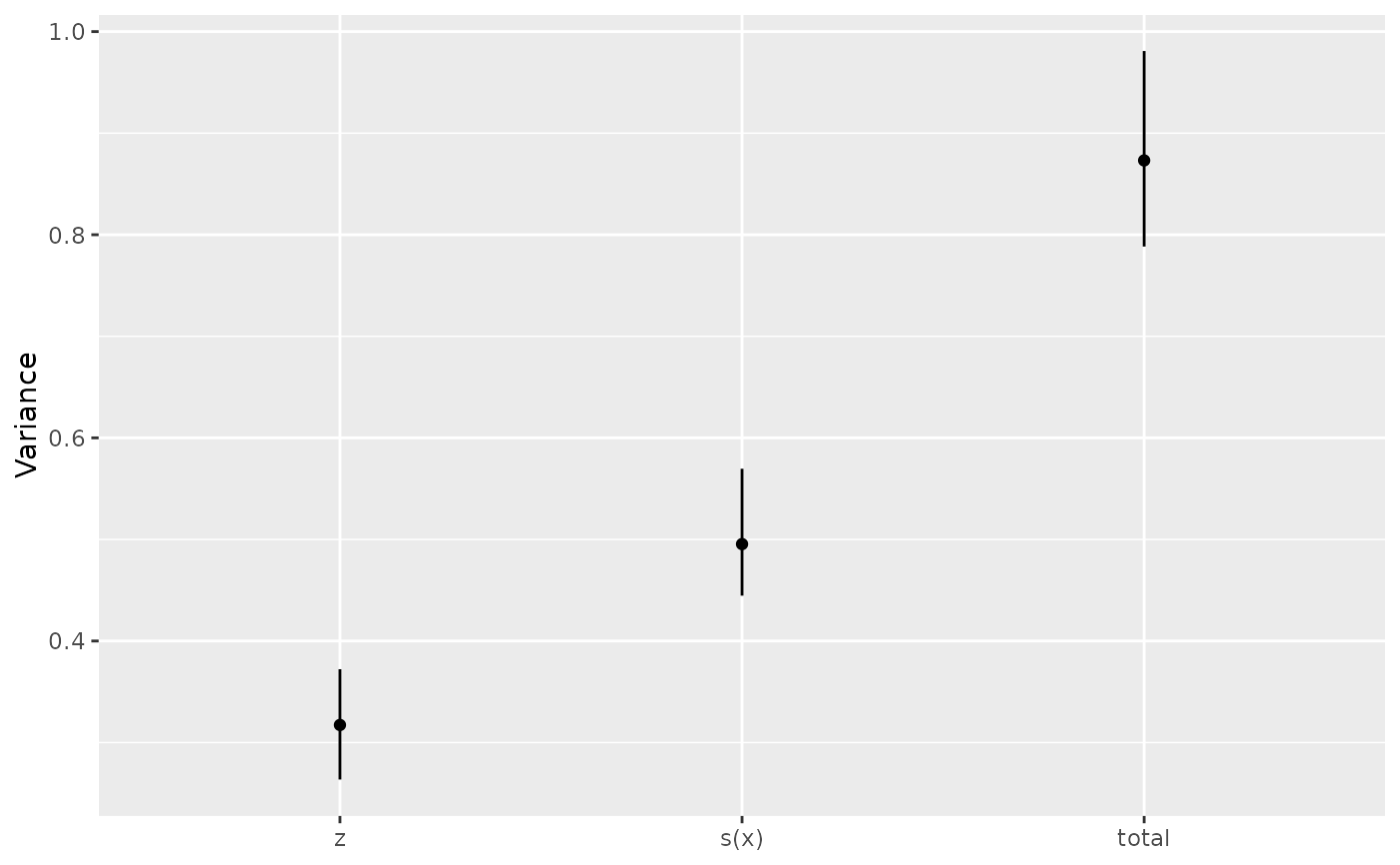
Plot variance components and proportions of term variance

Draw estimates and their stored confidence intervals, with components on the x-axis by default. No model fitting or posterior sampling is performed.

Usage

# S3 method for class 'variance_comp'
draw(
  object,
  type = c("variance", "std_dev", "proportion"),
  select = NULL,
  include_total = TRUE,
  predictor = NULL,
  ncol = NULL,
  nrow = NULL,
  angle = NULL,
  n_dodge = 1L,
  flip = FALSE,
  ...
)

Arguments

object: A result from variance_comp().
type: What to plot: "variance" (the default), "std_dev", or "proportion". Proportions require variance_comp(..., type = "terms").
select: Components to plot, as exact names, positive integer positions, or a logical vector with one entry per row of object. Components are displayed from left to right in the requested order, or from top to bottom with flip = TRUE. Use positions when component names are duplicated.
include_total: Logical; include the total rows of term results? Defaults to TRUE. Selection positions refer to object before totals are removed.
predictor: Linear predictors to plot for type = "proportion", as positive integer positions or total labels ("total", "total.1", and so on). The default plots all predictors, with separate panels when more than one is present. Shared terms appear in each relevant panel.
ncol, nrow: Number of columns or rows for the panels.
angle: Numeric; angle of the component labels in degrees, between -90 and 90. Passed to ggplot2::guide_axis(). The default, NULL, uses the angle specified by the plot theme.
n_dodge: Positive integer; number of rows for component labels, or columns with flip = TRUE. Use, for example, n_dodge = 2 to stagger labels that would overlap. Passed to the n.dodge argument of ggplot2::guide_axis(). Defaults to 1.
flip: Logical; put components on the y-axis? Defaults to FALSE.
...: Not used. Modify the returned plot with ggplot2 layers, scales and themes.

Value

A ggplot2::ggplot() object.

Details

Variance plots square the stored standard-deviation interval bounds so that estimates and intervals use the same scale. Standard-deviation and proportion plots use their stored bounds directly. Components with unavailable intervals retain their points. Intervals are drawn when both bounds are finite. Undefined estimates have no point, but retain their component labels.

Proportions can be negative or greater than one, and the plot preserves those values. Each panel shows only terms belonging to that predictor and its own total. A predictor with zero total variance has undefined proportions and is displayed without points or intervals.

Points use the geom.gratia.effect theme element and intervals use geom.gratia.interval; see gratia_theme_get().

Label layout

Pass label_control = draw_label_control(...) to draw() to wrap discrete axis labels and legend text, stagger discrete tick labels, or adjust legend and colour-bar layout. Settings apply to each panel, including unwrapped plot lists. See draw_label_control() for the available settings.

Examples

load_mgcv()
# Simulate linear and nonlinear effects with Gaussian noise
set.seed(42)
dat <- data.frame(x = runif(120), z = runif(120))
dat$y <- 2 * dat$z + sin(2 * pi * dat$x) + rnorm(120, sd = 0.3)

# Fit a linear effect of z and a smooth effect of x
model <- gam(y ~ z + s(x, k = 8), data = dat, method = "REML")

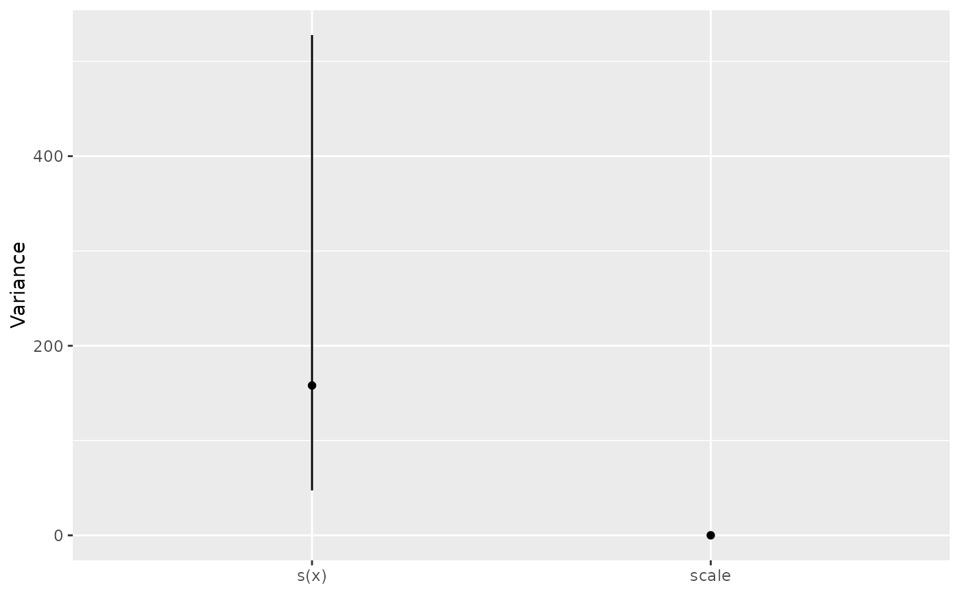
# Plot the variances used in the random-effect representation of the penalties
components <- variance_comp(model)
draw(components)


# Plot variation of fitted term contributions across the fitting observations
terms <- variance_comp(model, type = "terms", n_draws = 200, seed = 42)
draw(terms)