Create a ggplot Object

Function ordiggplot sets up an ordination graph but draws no result. You can add new graphical elements to this plot with geom_ordi_* functions of this package, or you can use standard ggplot2 geom_* functions and use ggscores as their data argument.

Usage

ordiggplot(model, axes = c(1, 2), legend.position = "right", ...)

ggscores(score)

Arguments

model: An ordination result object with a compatible fortify() meethods (typically from vegan).
axes: Two axes to be plotted
legend.position: Legend position: see ggplot2::theme() for details. Use "none" to not draw the legend. Some ggplot2::theme() can ignore this argument.
...: Parameters passed to fortify functions to extract ordination scores. You can define scores arguments such as scaling.
score: Ordination score to be added to the plot.

Value

Returns a ggplot object with slot data for full ordination data and slot mapping with ordination axes mapped to x and y, label to text labels for each row and factor score type mapped to colour.

Details

The ggvegan package has two contrasting approaches to draw ordination plots. The autoplot functions (e.g. autoplot.rda(), autoplot.cca(), and autoplot.metaMDS()) draw a complete plot with one command, but the design is hard-coded in the function, and it may be difficult to add new layers to the graph.

In contrast, function ordiggplot() only sets up an ordination plot, but allows you to add layers to the graph one by one with full flexibility of the ggplot2 functions. It initializes the ggplot2 graph with idiom ggplot(data, mapping) which allows other functions to use the ordination data and axis mapping in adding new layers. The included mapping specifies coordinates x and y and variables label for text labels and a score-type specific colour. Any ggplot2 function that can use this mapping will work automatically. Support function ggscores selects a slice of ordination scores that can be used as a data argument in the geom function. To plot the site scores of ordination result mod as points, you can use idiom ordiggplot(mod) + geom_point(data = ggscores("sites")).

There are specific functions to ease adding layers to an ordination graph. See the documentation of geom_ordi_arrow(), geom_ordi_label(), geom_ordi_point(), geom_ordi_repel(), geom_ordi_text(). These correspond to similarly named geom_* functions. For instance, geom_ordi_point adds very little to geom_point, and you can use all arguments of the standard geom function. These functions are of type geom_ordi_*(score, ...) which is similar to geom_*(data = ggscores(score), ...). Some functions were adapted to typical ordination data and return compound geometries. For instance, geom_ordi_arrow() returns layers geom_segment for the arrows, and geom_text for their name labels. In addition, there are functions to add previously fitted results of vegan::envfit() and vegan::ordisurf() (see autolayer.envfit(), autolayer.ordisurf()).

The ordiggplot() function extracts results using fortify() functions of this package, and it accepts the arguments of those functions. This allows setting, e.g., the scaling of ordination axes. The ordiggplot skeleton sets up data used in plotting, and you should define axis scaling, axes etc in the ordiggplot call and they will be used in all added layers.

Author

Jari Oksanen

Examples

library("vegan")
library("ggplot2")
data(dune, dune.env, varespec, varechem)
m <- cca(dune ~ Management + A1, dune.env)

## data and mapping of the ordiggplot object
ordiggplot(m)@data
#> # A tibble: 75 × 5
#>    score   label      cca1   cca2  weight
#>    <fct>   <chr>     <dbl>  <dbl>   <dbl>
#>  1 species Achimill  0.215  0.679 0.0234 
#>  2 species Agrostol -0.121 -0.757 0.0701 
#>  3 species Airaprae -1.84   0.888 0.00730
#>  4 species Alopgeni  0.538 -0.660 0.0526 
#>  5 species Anthodor -0.377  0.581 0.0307 
#>  6 species Bellpere  0.141  0.228 0.0190 
#>  7 species Bromhord  0.502  0.525 0.0219 
#>  8 species Chenalbu  0.522 -1.41  0.00146
#>  9 species Cirsarve  0.556 -0.667 0.00292
#> 10 species Comapalu -1.96  -1.84  0.00584
#> # ℹ 65 more rows
ordiggplot(m)@mapping
#> Aesthetic mapping: 
#> * `x`      -> `.data[["cca1"]]`
#> * `y`      -> `.data[["cca2"]]`
#> * `label`  -> `.data[["label"]]`
#> * `colour` -> `.data[["score"]]`

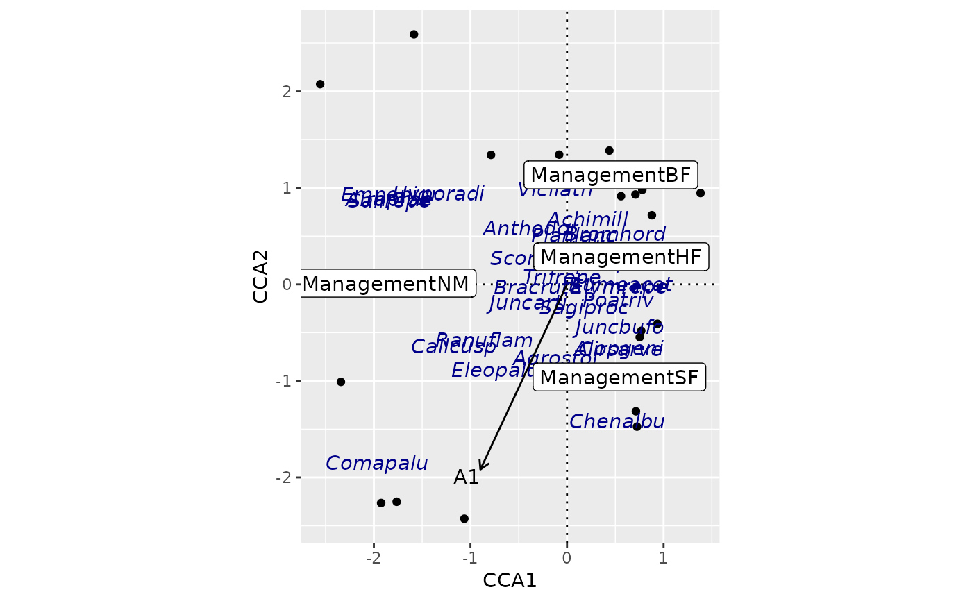
## use geom_ordi_* functions
ordiggplot(m) + geom_ordi_axis() +
  geom_ordi_point("sites") +
  geom_ordi_repel("species", col = "darkblue",
                 text.params = list(mapping = aes(fontface = "italic"))) +
  geom_ordi_label("centroids") +
  geom_ordi_arrow("biplot")


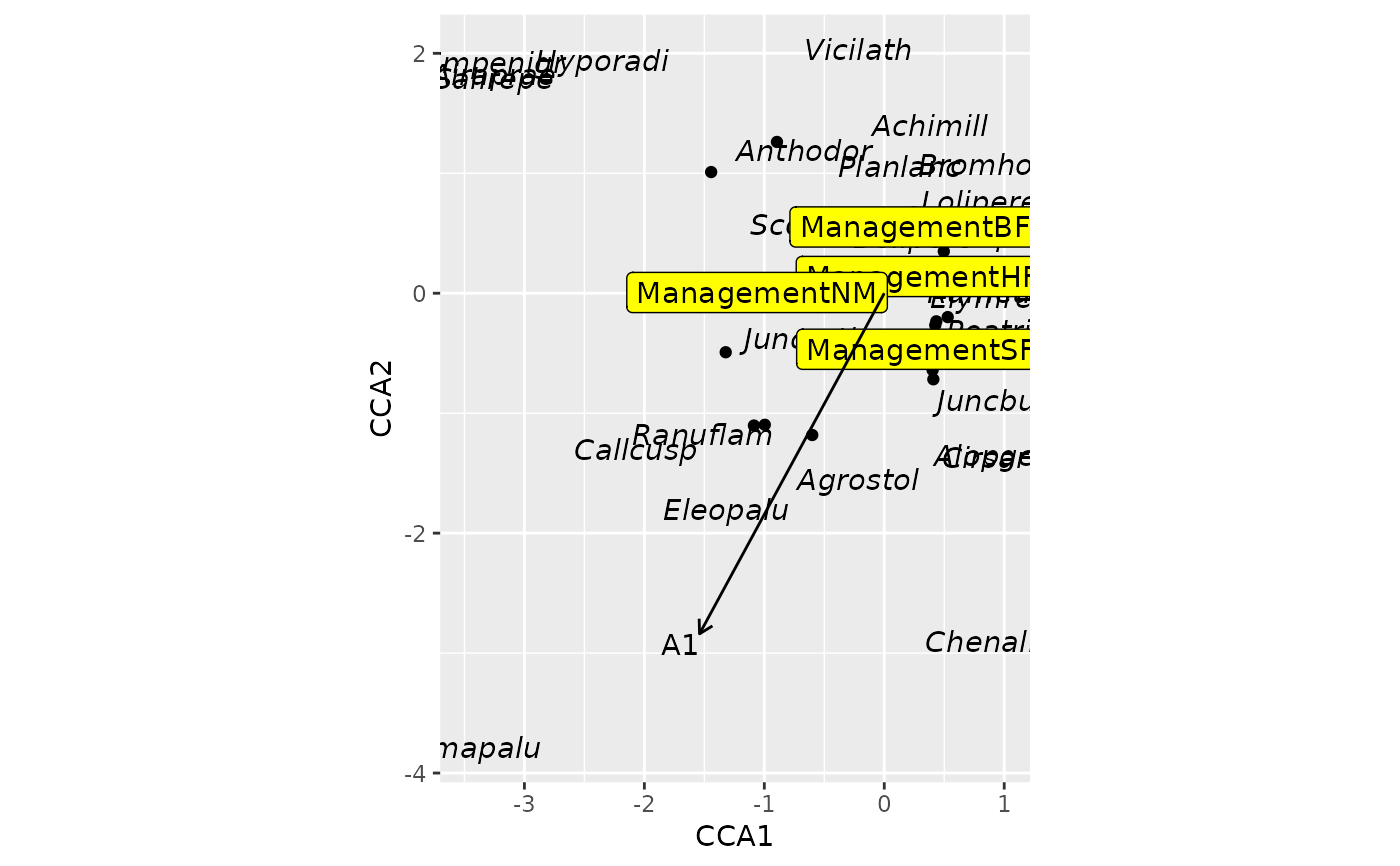
## use ggscores + standard geom_* functions
ordiggplot(m, scaling = "sites") +
  geom_point(data = ggscores("sites")) +
  geom_text(data = ggscores("species"),
            mapping = aes(fontface = "italic")) +
  geom_label(data = ggscores("centroids"), fill = "yellow") +
  geom_ordi_arrow("biplot")


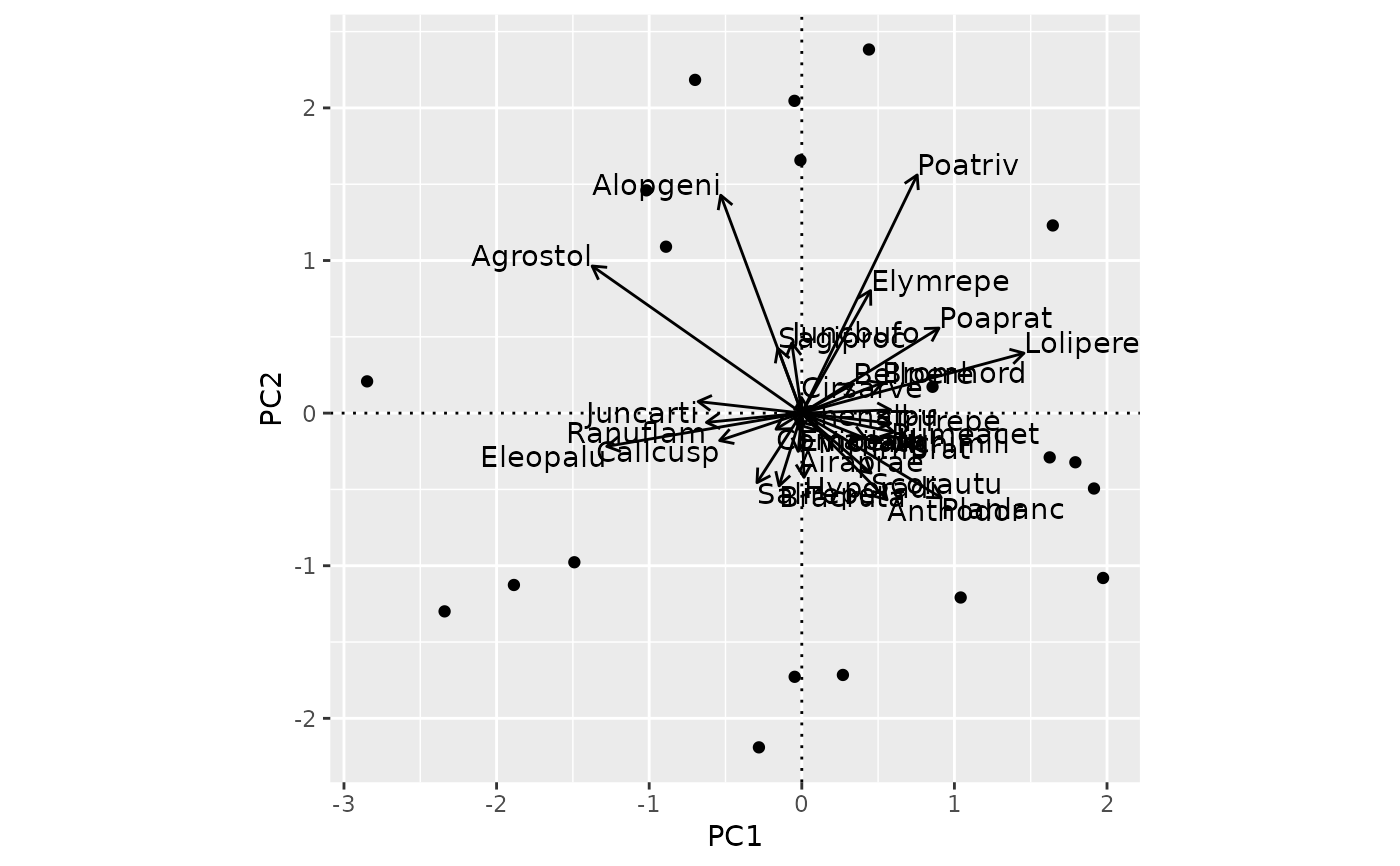
## Messy arrow biplot for PCA
m <- rda(dune)
ordiggplot(m, corr = TRUE) +
  geom_ordi_axis() +
  geom_ordi_point("sites") +
  geom_ordi_arrow("species")