Plot the result of a call to smooth_estimates()

Plot the result of a call to smooth_estimates()

Usage

# S3 method for class 'smooth_estimates'
draw(
  object,
  constant = NULL,
  fun = NULL,
  contour = TRUE,
  grouped_by = FALSE,
  contour_col = "black",
  n_contour = NULL,
  ci_alpha = 0.2,
  ci_col = "black",
  smooth_col = "black",
  resid_col = "steelblue3",
  decrease_col = "#56B4E9",
  increase_col = "#E69F00",
  change_lwd = 1.75,
  partial_match = FALSE,
  discrete_colour = NULL,
  discrete_fill = NULL,
  continuous_colour = NULL,
  continuous_fill = NULL,
  angle = NULL,
  ylim = NULL,
  crs = NULL,
  default_crs = NULL,
  lims_method = "cross",
  caption = TRUE,
  ...
)

Arguments

object

a fitted GAM, the result of a call to mgcv::gam().

constant

numeric; a constant to add to the estimated values of the smooth. constant, if supplied, will be added to the estimated value before the confidence band is computed.

fun

function; a function that will be applied to the estimated values and confidence interval before plotting. Can be a function or the name of a function. Function fun will be applied after adding any constant, if provided.

contour

logical; should contours be draw on the plot using ggplot2::geom_contour().

grouped_by

logical; should factor by smooths be drawn as one panel per level of the factor (FALSE, the default), or should the individual smooths be combined into a single panel containing all levels (TRUE)?

contour_col

colour specification for contour lines.

n_contour

numeric; the number of contour bins. Will result in n_contour - 1 contour lines being drawn. See ggplot2::geom_contour().

ci_alpha

numeric; alpha transparency for confidence or simultaneous interval.

ci_col

colour specification for the confidence/credible intervals band. Affects the fill of the interval.

smooth_col

colour specification for the smooth line.

resid_col

colour specification for the partial residuals.

decrease_col, increase_col

colour specifications to use for indicating periods of change. col_change is used when change_type = "change", while col_decrease and col_increase are used when `change_type = "sizer"“.

change_lwd

numeric; the value to set the linewidth to in ggplot2::geom_line(), used to represent the periods of change.

partial_match

logical; should smooths be selected by partial matches with select? If TRUE, select can only be a single string to match against.

discrete_colour

a suitable colour scale to be used when plotting discrete variables.

discrete_fill

a suitable fill scale to be used when plotting discrete variables.

continuous_colour

a suitable colour scale to be used when plotting continuous variables.

continuous_fill

a suitable fill scale to be used when plotting continuous variables.

angle

numeric; the angle at which the x axis tick labels are to be drawn passed to the angle argument of ggplot2::guide_axis().

ylim

numeric; vector of y axis limits to use all all panels drawn.

crs

the coordinate reference system (CRS) to use for the plot. All data will be projected into this CRS. See ggplot2::coord_sf() for details.

default_crs

the coordinate reference system (CRS) to use for the non-sf layers in the plot. If left at the default NULL, the CRS used is 4326 (WGS84), which is appropriate for spline-on-the-sphere smooths, which are parameterized in terms of latitude and longitude as coordinates. See ggplot2::coord_sf() for more details.

lims_method

character; affects how the axis limits are determined. See ggplot2::coord_sf(). Be careful; in testing of some examples, changing this to "orthogonal" for example with the chlorophyll-a example from Simon Wood's GAM book quickly used up all the RAM in my test system and the OS killed R. This could be incorrect usage on my part; right now the grid of points at which SOS smooths are evaluated (if not supplied by the user) can produce invalid coordinates for the corners of tiles as the grid is generated for tile centres without respect to the spacing of those tiles.

caption

logical; show the smooth type in the caption of each plot?

...

additional arguments passed to patchwork::wrap_plots().

Examples

load_mgcv()
# example data
df <- data_sim("eg1", seed = 21)
# fit GAM
m <- gam(y ~ s(x0) + s(x1) + s(x2) + s(x3), data = df, method = "REML")
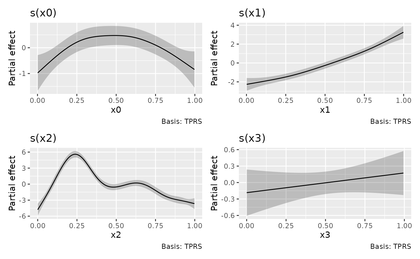
# plot all of the estimated smooths
sm <- smooth_estimates(m)
draw(sm)

# evaluate smooth of `x2`
sm <- smooth_estimates(m, select = "s(x2)")
# plot it
draw(sm)


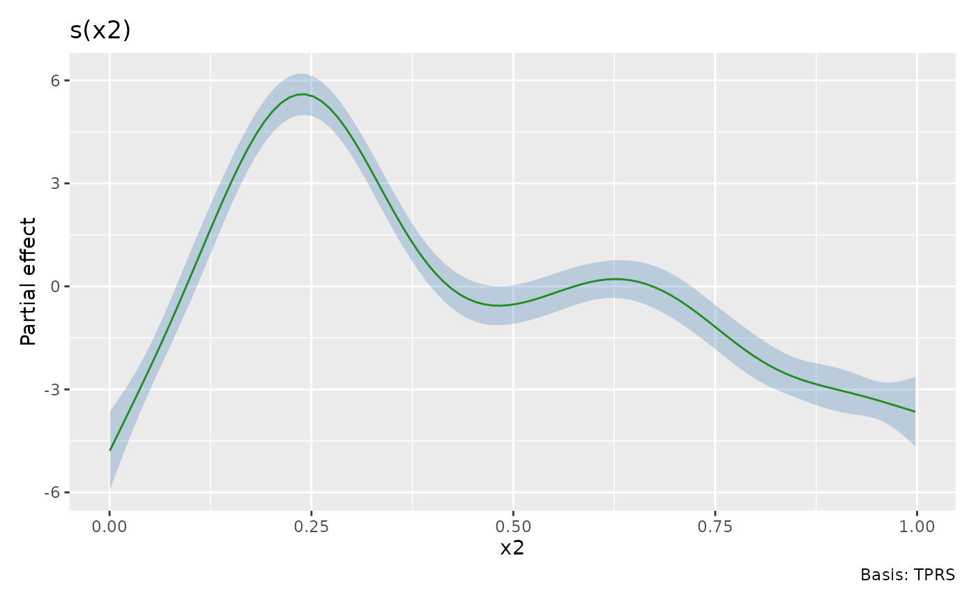
# customising some plot elements
draw(sm, ci_col = "steelblue", smooth_col = "forestgreen", ci_alpha = 0.3)


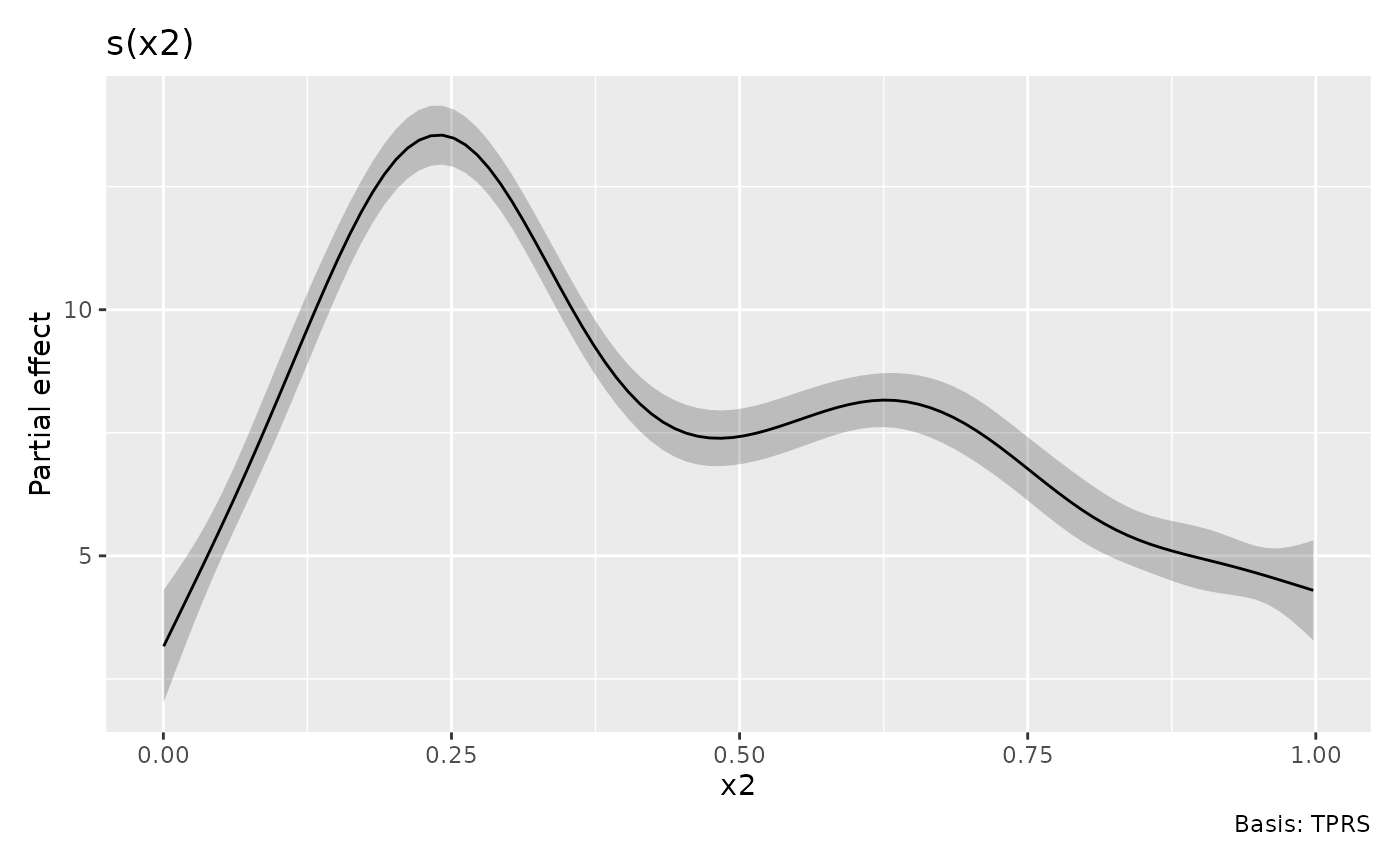
# Add a constant to the plotted smooth
draw(sm, constant = coef(m)[1])


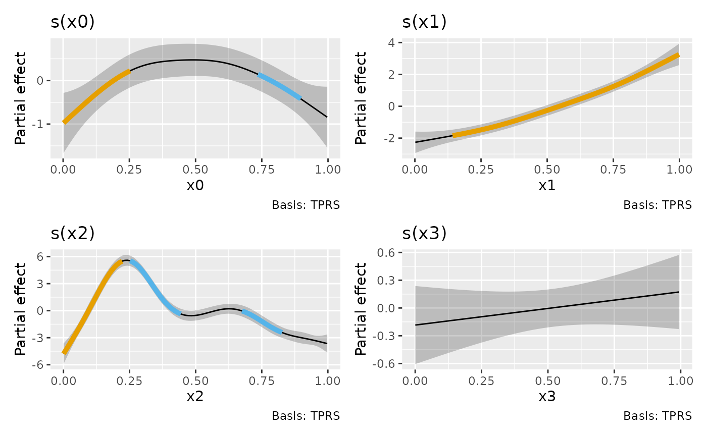
# Adding change indicators to smooths based on derivatives of the smooth
d <- derivatives(m, n = 100) # n to match smooth_estimates()

smooth_estimates(m) |>
  add_sizer(derivatives = d, type = "sizer") |>
  draw()