Plot smooths of a GAMLSS model estimated by GJRM::gamlss

Provides a draw() method for GAMLSS (distributional GAMs) fitted by GJRM::gamlss().

Usage

# S3 method for class 'gamlss'
draw(
  object,
  scales = c("free", "fixed"),
  ncol = NULL,
  nrow = NULL,
  guides = "keep",
  widths = NULL,
  heights = NULL,
  ...
)

Arguments

object

a model, fitted by GJRM::gamlss()

scales

character; should all univariate smooths be plotted with the same y-axis scale? If scales = "free", the default, each univariate smooth has its own y-axis scale. If scales = "fixed", a common y axis scale is used for all univariate smooths.

Currently does not affect the y-axis scale of plots of the parametric terms.

ncol, nrow

numeric; the numbers of rows and columns over which to spread the plots

guides

character; one of "keep" (the default), "collect", or "auto". Passed to patchwork::plot_layout()

widths, heights

The relative widths and heights of each column and row in the grid. Will get repeated to match the dimensions of the grid. If there is more than 1 plot and widths = NULL, the value of widths will be set internally to widths = 1 to accommodate plots of smooths that use a fixed aspect ratio.

...

arguments passed to draw.gam()

Note

Plots of smooths are not labelled with the linear predictor to which they belong.

Examples

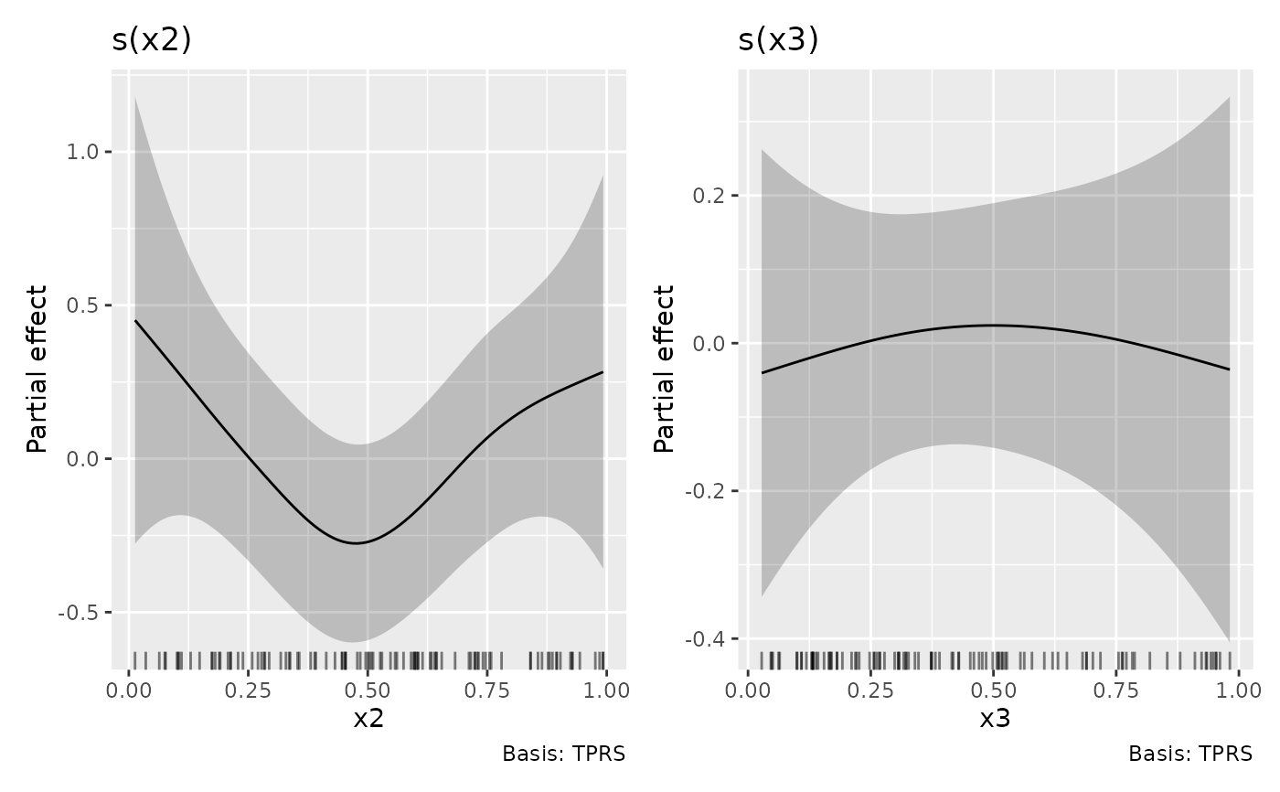
if (suppressPackageStartupMessages(require("GJRM", quietly = TRUE))) {
  # follow example from ?GJRM::gamlss
  load_mgcv()
  suppressPackageStartupMessages(library("GJRM"))
  set.seed(0)
  n <- 100
  x1 <- round(runif(n))
  x2 <- runif(n)
  x3 <- runif(n)
  f1 <- function(x) cos(pi * 2 * x) + sin(pi * x)
  y1 <- -1.55 + 2 * x1 + f1(x2) + rnorm(n)
  dataSim <- data.frame(y1, x1, x2, x3)

  eq_mu <- y1 ~ x1 + s(x2)
  eq_s <- ~ s(x3, k = 6)
  fl <- list(eq_mu, eq_s)
  m <- gamlss(fl, data = dataSim)

  draw(m)
}