Posterior expectations of derivatives from an estimated model

Usage

derivative_samples(object, ...)

# Default S3 method
derivative_samples(object, ...)

# S3 method for class 'gamm'
derivative_samples(object, ...)

# S3 method for class 'gam'
derivative_samples(
  object,
  focal = NULL,
  data = NULL,
  order = 1L,
  type = c("forward", "backward", "central"),
  scale = c("response", "linear_predictor"),
  method = c("gaussian", "mh", "inla", "user"),
  n = 100,
  eps = NULL,
  n_sim = 10000,
  level = lifecycle::deprecated(),
  seed = NULL,
  envir = environment(formula(object)),
  draws = NULL,
  mvn_method = c("mvnfast", "mgcv"),
  ...
)

# S3 method for class 'scam'
derivative_samples(
  object,
  focal = NULL,
  data = NULL,
  order = 1L,
  type = c("forward", "backward", "central"),
  scale = c("response", "linear_predictor"),
  method = c("gaussian", "mh", "inla", "user"),
  n = 100,
  eps = NULL,
  n_sim = 10000,
  seed = NULL,
  envir = environment(formula(object)),
  draws = NULL,
  mvn_method = c("mvnfast", "mgcv"),
  ...
)

Arguments

object: an R object to compute derivatives for
...: arguments passed to other methods and on to fitted_samples()
focal: character; name of the focal variable. The response derivative of the response with respect to this variable will be returned. All other variables involved in the model will be held at constant values. This must be supplied.
data: a data frame containing the values of the model covariates at which to evaluate derivatives of fitted values. If supplied, all but one variable must be held at a constant value.
order: numeric; the order of derivative.
type: character; the type of finite difference used. One of "forward", "backward", or "central".
scale: character; should the derivative be estimated on the response or the linear predictor (link) scale? One of "response" (the default), or "linear_predictor".
method: character; which method should be used to draw samples from the posterior distribution. "gaussian" uses a Gaussian (Laplace) approximation to the posterior. "mh" uses a Metropolis Hastings sample that alternates t proposals with proposals based on a shrunken version of the posterior covariance matrix. "inla" uses a variant of Integrated Nested Laplace Approximation due to Wood (2019), (currently not implemented). "user" allows for user-supplied posterior draws via draws in ....
n: numeric; the number of points to evaluate the derivative at (if data is not supplied).
eps: a positive finite number giving the absolute finite-difference step, or NULL (the default) to choose it automatically. The automatic step is the fitted range of the differentiation coordinate multiplied by .Machine$double.eps^(1 / (order + p)), where p = 2 for central differences and p = 1 for forward or backward differences. A constant coordinate uses its absolute value (or one if zero) instead of its range. The step is rounded upwards and bounded below so that adding it to the coordinates produces a representable change. Stored transformed values or raw covariate summaries supply the range; supplied data are used if neither is available. This is a scale-aware heuristic, not an error bound; unusual function scales or domain boundaries may require explicit eps. For first central differences the two points are separated by eps; for second central differences they are each eps from the target.
n_sim: integer; number of posterior draws. Ignored when using user-supplied draws.
level
seed: numeric; a random seed for the simulations.
envir: the environment within which to recreate the data used to fit object.
draws: matrix; user supplied posterior draws to be used when method = "user".
mvn_method: character; one of "mvnfast" or "mgcv". The default is uses mvnfast::rmvn(), which can be considerably faster at generate large numbers of MVN random values than mgcv::rmvn(), but which might not work for some marginal fits, such as those where the covariance matrix is close to singular.

Value

A tibble, currently with the following variables:

.derivative: the estimated partial derivative,
additional columns containing the covariate values at which the derivative was evaluated.

Author

Gavin L. Simpson

Examples


load_mgcv()
df <- data_sim("eg1", dist = "negbin", scale = 0.25, seed = 42)

# fit the GAM (note: for execution time reasons using bam())
m <- bam(y ~ s(x0) + s(x1) + s(x2) + s(x3),
  data = df, family = nb(), method = "fREML")

# data slice through data along x2 - all other covariates will be set to
# typical values (value closest to median)
ds <- data_slice(m, x2 = evenly(x2, n = 200))

# samples from posterior of derivatives
fd_samp <- derivative_samples(m,
  data = ds, type = "central",
  focal = "x2", eps = 0.01, seed = 21, n_sim = 100
)

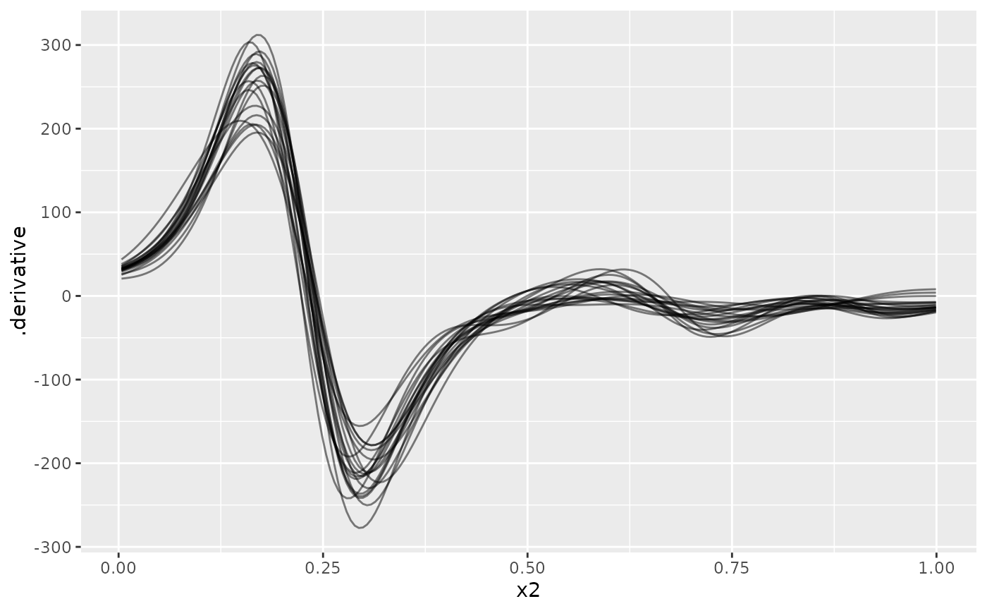
# plot the first 20 posterior draws
if (requireNamespace("ggplot2") && requireNamespace("dplyr")) {
  library("ggplot2")
  fd_samp |>
    dplyr::filter(.draw <= 20) |>
    ggplot(aes(x = x2, y = .derivative, group = .draw)) +
    geom_line(alpha = 0.5)
}