Compare smooths across models

Usage

compare_smooths(
  model,
  ...,
  select = NULL,
  smooths = deprecated(),
  n = 100,
  n_2d = 50,
  data = NULL,
  unconditional = FALSE,
  overall_uncertainty = TRUE,
  partial_match = FALSE,
  envir = NULL,
  dist = NULL
)

Arguments

model: Primary model for comparison.
...: Additional models to compare smooths against those of model.
select: character; select which smooths to compare. The default (NULL) means all smooths in model will be compared. Numeric select indexes the smooths in the order they are specified in the formula and stored in model. Character select matches the labels for smooths as shown for example in the output from summary(object). Logical select operates as per numeric select in the order that smooths are stored.
smooths: Use select instead.
n: numeric; the number of points over the range of the covariate at which to evaluate a univariate smooth.
n_2d: numeric; the number of points along each of the first two axes of a smooth surface, including surface panels of higher-dimensional smooths. The default is 50 in plotting and plot-preparation functions. If NULL, use n instead. Ignored when evaluation data are supplied. Factor levels are retained, and curves with only one continuous covariate use n.
data: a data frame of covariate values at which to evaluate the smooth.
unconditional: logical; if TRUE (and only if frequentist == FALSE) then the bayesian smoothing parameter uncertainty-corrected covariance matrix is returned, if available. Whether it is available depends on which smoothness selection method was used to fit the model.
overall_uncertainty: logical; should the uncertainty in the model constant term be included in the standard error of the evaluate values of the smooth?
partial_match: logical; should smooths be selected by partial matches with select? If TRUE, select can only be a single string to match against.
envir: an optional environment supplying functions and constants used in model expressions. The available model formula environment is used when NULL. Covariate observations should be supplied in data.
dist: numeric; if greater than 0, this is used to determine when a location is too far from data to be plotted when plotting 2-D smooths. The data are scaled into the unit square before deciding what to exclude, and dist is a distance within the unit square. See mgcv::exclude.too.far() for further details.

Details

Two-variable smooths are evaluated at common locations. Automatic grids span the intersection of the models' observed covariate ranges; factor levels must overlap. Supplied data are evaluated as given, without filling gaps. Each selected smooth label must occur exactly once in every model and use the same covariates, including any by variable. Numeric and logical select refer to the primary model; matching labels are then used in every model.

Estimates are contributions of individual smooths to the linear predictor, on its link scale, with the centring constraints used in each fitted model. They exclude the intercept and other model terms. Different fitting data can change the centring, so a surface difference can include a constant shift. It is the difference between these fitted smooth contributions, rather than a difference between fitted responses.

The result retains one row per model and smooth, with estimates in the data list column. For distributional models, .parameter retains the label for the linear predictor, while .model identifies the input model. Use draw.compare_smooths() for faceted surface comparisons or estimated surface differences. Smooths with more than two covariates can be evaluated but cannot be drawn by this method.

Examples

load_mgcv()
dat <- data_sim("eg1", seed = 2)

## models to compare smooths across - artificially create differences
m1 <- gam(y ~ s(x0, k = 5) + s(x1, k = 5) + s(x2, k = 5) + s(x3, k = 5),
  data = dat, method = "REML"
)
m2 <- gam(y ~ s(x0, bs = "ts") + s(x1, bs = "ts") + s(x2, bs = "ts") +
  s(x3, bs = "ts"), data = dat, method = "REML")

## build comparisons
comp <- compare_smooths(m1, m2)
comp
#> # A tibble: 8 x 5
#>   .model .smooth .type         .by   data              
#>   <chr>  <chr>   <chr>         <chr> <list>            
#> 1 m1     s(x0)   TPRS          NA    <tibble [100 x 3]>
#> 2 m2     s(x0)   TPRS (shrink) NA    <tibble [100 x 3]>
#> 3 m1     s(x1)   TPRS          NA    <tibble [100 x 3]>
#> 4 m2     s(x1)   TPRS (shrink) NA    <tibble [100 x 3]>
#> 5 m1     s(x2)   TPRS          NA    <tibble [100 x 3]>
#> 6 m2     s(x2)   TPRS (shrink) NA    <tibble [100 x 3]>
#> 7 m1     s(x3)   TPRS          NA    <tibble [100 x 3]>
#> 8 m2     s(x3)   TPRS (shrink) NA    <tibble [100 x 3]>
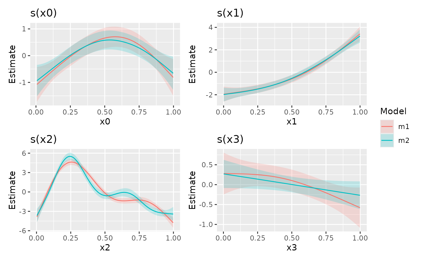
## notice that the result is a nested tibble

draw(comp)


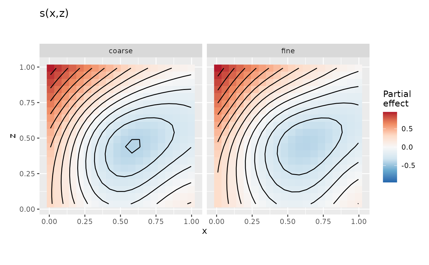
# Simulate a noisy response over two continuous covariates, x and z
surf <- data_sim("eg2", n = 100, seed = 7)
# Fit two small bases to the same surface data
coarse <- gam(y ~ s(x, z, k = 10), data = surf, method = "REML")
fine <- gam(y ~ s(x, z, k = 15), data = surf, method = "REML")
# Compare surfaces on shared axes and a shared colour scale
surfaces <- compare_smooths(coarse, fine, n_2d = 20)
draw(surfaces)

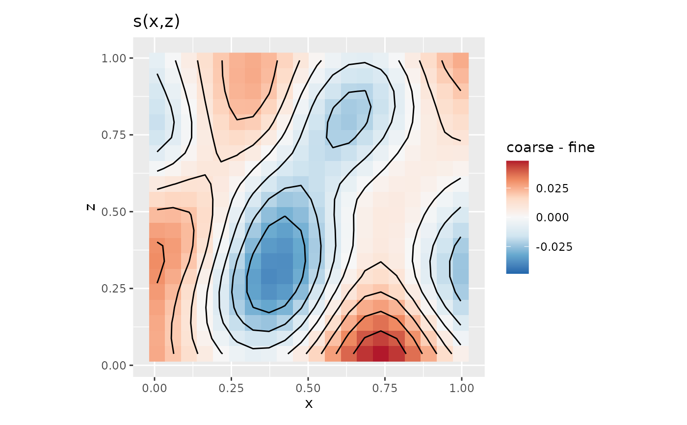
# Show coarse minus fine, with a colour scale centred on zero
draw(surfaces, show = "difference", pair = c("coarse", "fine"))