Fit an environmental vector or factor to a Co-CA ordination

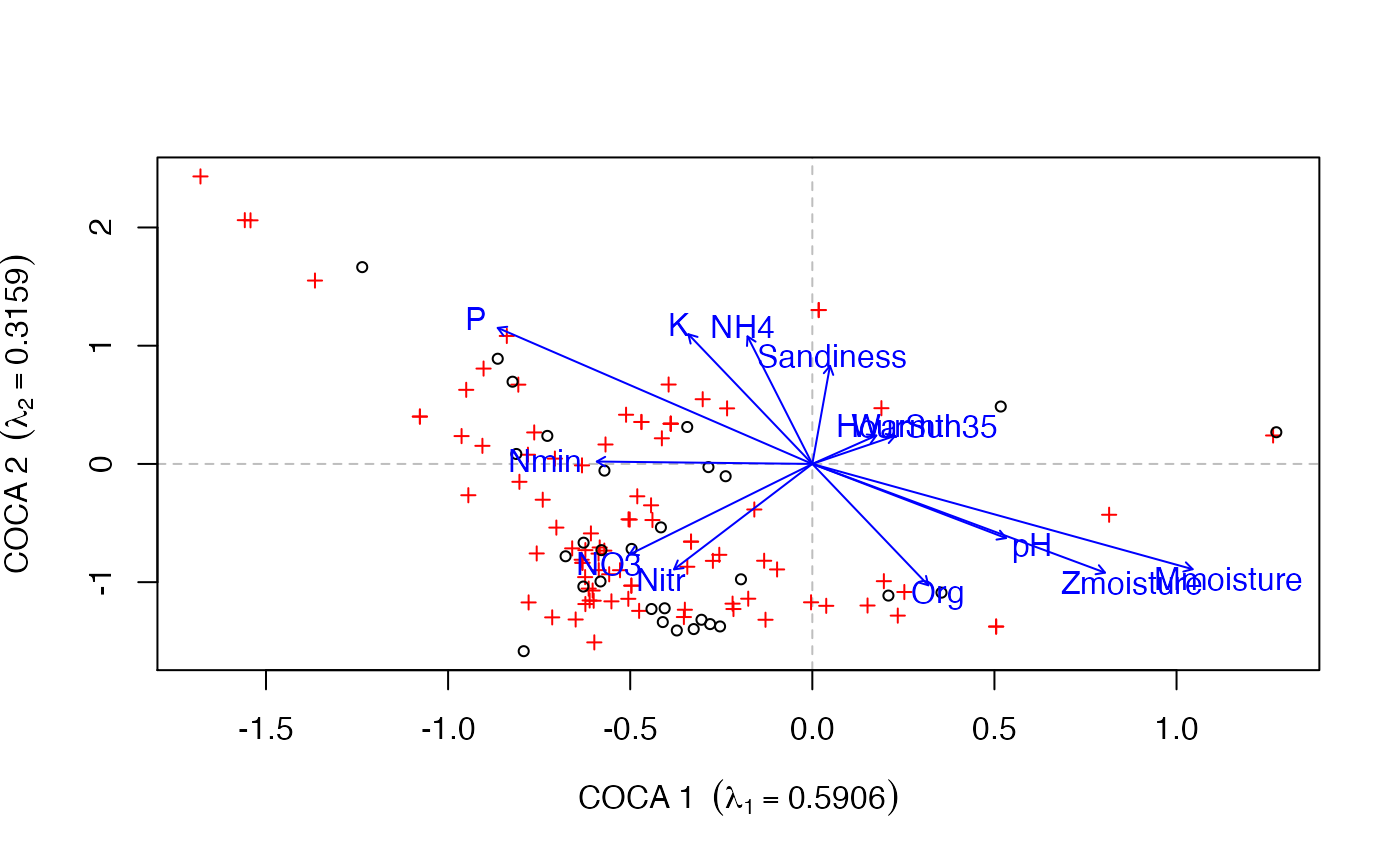
The function fits environmental vectors or factors to a Co-CA ordination. The projections of points onto vectors have maximum correlation with corresponding environmental variables, and the factors show the averages of factor levels.

# S3 method for coca
envfit(ord, env, which = c("response", "predictor"),
       choices = c(1, 2), scaling = FALSE, w, na.rm = FALSE,
       strata = NULL, permutations = 999, ...)

Arguments

ord	a Co-CA ordination object, the result of a call to coca.
env	a data frame, matrix or vector of environmental/external variable(s) to be fitted to the ordination. The variables may be of a mixed type (factors and continuous variables) in a data frame.
which	character; which of the response or predictor ordinations should be used during fitting of vectors and factors.
choices	numeric; the axes to which vectors and factors are fitted.
scaling	logical; should sacling be applied. See scores.symcoca.
w	weights used in fitting vectors and factors.
na.rm	Remove points with missing values in ordination scores or environmental variables. The operation is casewise; the whole row of data is removed if there is a missing value and na.rm = TRUE.
strata	An integer vector or factor specifying the strata for permutation. If supplied, observations are permuted only within the specified strata.
permutations	Number of permutations for assessing significance of vectors or factors. Set to 0 to skip permutations.
...	Arguments passed to vectorfit and factorfit.

Details

See envfit for details of the method.

Value

Returns an object of class envfit.

Author

Gavin L. Simpson. The code interfaces with and uses code from envfit for the main computations, which was written by Jari Oksanen.

See also

coca for fitting models. envfit for details of the generic function and the computations performed.

Examples

## symmetric CoCA
data(beetles)
data(plants)

## log transform the bettle data
beetles <- log(beetles + 1)

## fit the model
bp.sym <- coca(beetles ~ ., data = plants, method = "symmetric")
#> 
#> Removed some species that contained no data in: beetles, plants 

## load the environmental data
data(verges)

## fit vectors for the environmental data
sol <- envfit(bp.sym, verges, which = "response")
sol
#> 
#> ***VECTORS
#> 
#>             COCA 1   COCA 2     r2 Pr(>r)  
#> Mmoisture  0.76095 -0.64881 0.4686  0.036 *
#> Zmoisture  0.65812 -0.75292 0.3711  0.076 .
#> Org        0.29636 -0.95508 0.2873  0.162  
#> Sandiness  0.05840  0.99829 0.1718  0.422  
#> pH         0.64658 -0.76284 0.1683  0.490  
#> NO3       -0.54818 -0.83636 0.2088  0.294  
#> NH4       -0.16274  0.98667 0.2975  0.181  
#> Nmin      -0.99942  0.03412 0.0872  0.678  
#> P         -0.60030  0.79978 0.5153  0.034 *
#> K         -0.29634  0.95508 0.3284  0.114  
#> Nitr      -0.39179 -0.92005 0.2336  0.274  
#> HourSun    0.59022  0.80724 0.0220  0.878  
#> Warmth35   0.69088  0.72297 0.0269  0.833  
#> ---
#> Signif. codes:  0 ‘***’ 0.001 ‘**’ 0.01 ‘*’ 0.05 ‘.’ 0.1 ‘ ’ 1
#> Permutation: free
#> Number of permutations: 999
#> 
#> 

## plot the response matrix and the fitted vectors
biplot(bp.sym, which = "y1")
plot(sol)