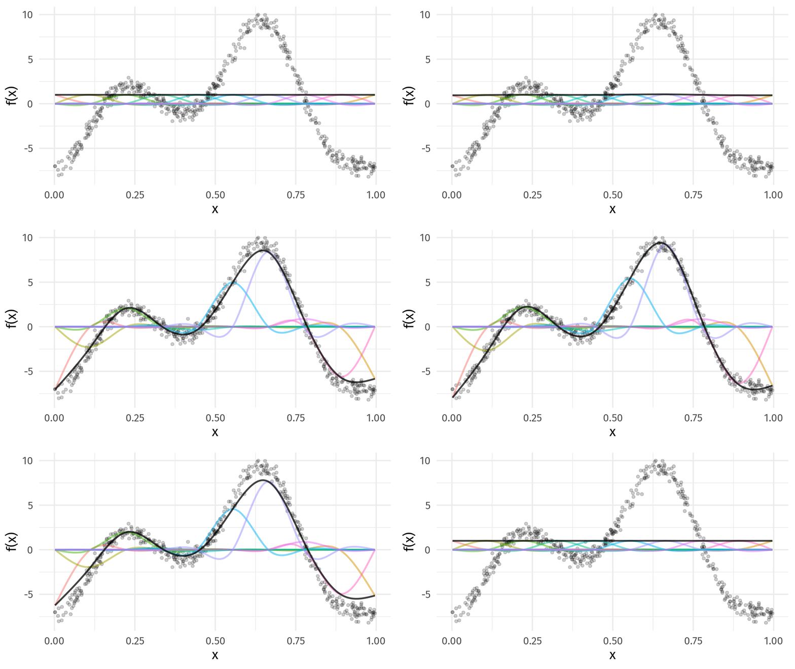
class: inverse, middle, left, my-title-slide, title-slide # Estimating the time-varying correlation between time series using copula distributional models ### Gavin Simpson ### vISEC2020 • June 22-26 2020 --- class: inverse middle center big-subsection # Correlation ??? Correlation: one of the first things we learn in undergraduate applied statistics Correlation is an intuitive way to think how the values of one variable vary with another How does the correlation between random variable change over time? --- class: inverse middle center large-subsection # Bivariate Copula Distributional GAM ??? Here I'll briefly explain how we've approached this question using a bivariate copula distributional GAM --- class: inverse middle center huge-subsection # Bivariate --- class: inverse middle center huge-subsection # Copulas --- # Copulas Function representing a joint distribution as a mapping from the CDFs of its marginals Defines a general way to think about *dependence* between random variables Starting to be used in ecology: * Popovic, Hui, Warton, 2018. *J. Multivar. Anal.* **165**, 86–100. [doi: 10/dzx9](http://doi.org/dzx9) * Anderson *et al* 2019. *Ecol. Evol.* **44**, 182. [doi: 10/dzzb](http://doi.org/dzzb) --- ## Copulas <!-- --> --- class: inverse middle center big-subsection # Distributional Regression --- # Model effects beyond the mean Complex data often can't be modelled as conditional means + a mean-variance relationship Distributional regression models have linear predictors for all parameters of the conditional distribution `$$\mathbf{y} | \vartheta^{k}$$` For a Gaussian response `$$\begin{align} \mu_i & = \beta^{\mu}_0 + \boldsymbol{x}_i^{\mathsf{T}}\boldsymbol{\beta}^{\mu}_j \\ \log(\sigma_i) & = \beta^{\sigma}_0 + \boldsymbol{x}_i^{\mathsf{T}}\boldsymbol{\beta}^{\sigma}_j \end{align}$$` --- class: inverse middle center massive-subsection # GAMs --- # Maximise penalised log-likelihood ⇨ β .center[] ??? Fitting a GAM involves finding the weights for the basis functions that produce a spline that fits the data best, subject to some constraints --- class: inverse middle center large-subsection # Bivariate + Copula + Distributional + GAM --- class: inverse middle center big-subsection # Example --- # Lake 227 Algal pigments well preserved in lake sediments * Reflect phytoplankton standing crops in lakes * Chlorophyll-*a* tracks planktonic sources * β-carotene tracks planktonic & benthic sources <!-- --> --- # Lake 227 Gaussian copula with Gamma univariate marginal responses .small[ `$$\begin{align} F(y_{\mathsf{Chl a}_{i}}, y_{\mathsf{\beta caro}_{i}} | \vartheta^{k} ) & = \mathcal{C}(F_{\mathsf{Chl a}_{i}}(y_{\mathsf{Chl a}_{i}} | \mu_{\mathsf{Chl a}_{i}}, \sigma_{\mathsf{Chl a}_{i}}), F_{\mathsf{\beta caro}_{i}}(y_{\mathsf{\beta caro}_{i}} | \mu_{\mathsf{\beta caro}_{i}}, \sigma_{\mathsf{\beta caro}_{i}}), \theta) \\ y_{\mathsf{Chl a}_{i}} & \sim \mathsf{Gamma}(\mu_{\mathsf{Chl a}_{i}}, \sigma_{\mathsf{Chl a}_{i}}) \\ y_{\mathsf{\beta caro}_{i}} & \sim \mathsf{Gamma}(\mu_{\mathsf{\beta caro}_{i}}, \sigma_{\mathsf{\beta caro}_{i}}) \end{align}$$` ] `$$\begin{align} \log(\mu_{\mathsf{Chl a}_{i}}) & = \beta^{\mu_{\mathsf{Chl a}}}_0 + f^{\mu_{\mathsf{Chl a}}}(\text{Year}_i) \\ \log(\mu_{\mathsf{\beta caro}_{i}}) & = \beta^{\mu_{\mathsf{\beta caro}}}_0 + f^{\mu_{\mathsf{\beta caro}}}(\text{Year}_i) \\ \log(\sigma_{\mathsf{Chl a}_{i}}) & = \beta^{\sigma_{\mathsf{Chl a}}}_0 \\ \log(\sigma_{\mathsf{\beta caro}_{i}}) & = \beta^{\sigma_{\mathsf{\beta caro}}}_0 \\ g(\theta_i) & = \beta^{\theta}_0 + f^{\theta}(\text{Year}_i) \end{align}$$` --- # Lake 227 Model Fitting Fitted with `gjrm()` from **GJRM ** package Marra, G., Radice, R., 2017. *Comput. Stat. Data Anal.* **112**, 99–113. [doi: 10/dzzc](http://doi.org/dzzc) --- # Lake 227 — μ Fitted mean functions for each response <!-- --> --- # Lake 227 — Kendall's τ Estimate `\(\theta\)` but can transform to Kendall's τ <!-- --> --- # Acknowledgements ### Funding .row[ .col-6[ .center[] ] .col-6[ .center[] ] ] ### Data Lake 227 data from Peter Leavitt (U Regina) ### Slides * HTML Slide deck [bit.ly/visec-copula-gam](http://bit.ly/visec-copula-gam) © Simpson (2020) [](http://creativecommons.org/licenses/by/4.0/) * RMarkdown [Source](https://github.com/gavinsimpson/visec-2020-copula-gam)