class: inverse, middle, left, my-title-slide, title-slide .title[ # Generalized Additive Models ] .subtitle[ ## a data-driven approach to estimating regression models ] .author[ ### Gavin Simpson ] .institute[ ### Department of Animal & Veterinary Sciences · Aarhus University ] .date[ ### 1400–2000 CET (1300–1900 UTC) Tuesday 9th December, 2025 ] --- class: inverse middle center big-subsection # Welcome ??? --- # Logistics ## Slides Slidedeck: [bit.ly/physalia-gam-2](https://bit.ly/physalia-gam-2) Sources: [bit.ly/physalia-gam](https://bit.ly/physalia-gam) --- # Today's topics * How do GAMs work? * What are splines? * How do GAMs learn from data without overfitting? --- class: inverse middle center huge-subsection # GAMs --- class: inverse middle center subsection # Motivating example --- # HadCRUT4 time series <!-- --> ??? Hadley Centre NH temperature record ensemble How would you model the trend in these data? --- # (Generalized) Linear Models `$$y_i \sim \mathcal{N}(\mu_i, \sigma^2)$$` `$$\mu_i = \beta_0 + \beta_1 \mathtt{year}_{i} + \beta_2 \mathtt{year}^2_{1i} + \cdots + \beta_j \mathtt{year}^j_{i}$$` Assumptions 1. linear effects of covariates are good approximation of the true effects 2. conditional on the values of covariates, `\(y_i | \mathbf{X} \sim \mathcal{N}(\mu_i, \sigma^2)\)` 3. this implies all observations have the same *variance* 4. `\(y_i | \mathbf{X} = \mathbf{x}\)` are *independent* An **additive** model addresses the first of these --- class: inverse center middle subsection # Why bother with anything more complex? --- # Is this linear? <!-- --> --- # Polynomials perhaps… <!-- --> --- # Polynomials perhaps… We can keep on adding ever more powers of `\(\boldsymbol{x}\)` to the model — model selection problem **Runge phenomenon** — oscillations at the edges of an interval — means simply moving to higher-order polynomials doesn't always improve accuracy --- class: inverse middle center subsection # GAMs offer a solution --- # HadCRUT data set ``` r library("readr") library("dplyr") URL <- "https://bit.ly/hadcrutv4" gtemp <- read_table( URL, col_types = "nnnnnnnnnnnn", col_names = FALSE ) |> select(num_range("X", 1:2)) |> setNames(nm = c("Year", "Temperature")) ``` [File format](https://www.metoffice.gov.uk/hadobs/hadcrut4/data/current/series_format.html) --- # HadCRUT data set ``` r gtemp ``` ``` ## # A tibble: 172 × 2 ## Year Temperature ## <dbl> <dbl> ## 1 1850 -0.336 ## 2 1851 -0.159 ## 3 1852 -0.107 ## 4 1853 -0.177 ## 5 1854 -0.071 ## 6 1855 -0.19 ## 7 1856 -0.378 ## 8 1857 -0.405 ## 9 1858 -0.4 ## 10 1859 -0.215 ## # ℹ 162 more rows ``` --- # Fitting a GAM ``` r library("mgcv") m <- gam(Temperature ~ s(Year), data = gtemp, method = "REML") summary(m) ``` .smaller[ ``` ## ## Family: gaussian ## Link function: identity ## ## Formula: ## Temperature ~ s(Year) ## ## Parametric coefficients: ## Estimate Std. Error t value Pr(>|t|) ## (Intercept) -0.020477 0.009731 -2.104 0.0369 * ## --- ## Signif. codes: 0 '***' 0.001 '**' 0.01 '*' 0.05 '.' 0.1 ' ' 1 ## ## Approximate significance of smooth terms: ## edf Ref.df F p-value ## s(Year) 7.837 8.65 145.1 <2e-16 *** ## --- ## Signif. codes: 0 '***' 0.001 '**' 0.01 '*' 0.05 '.' 0.1 ' ' 1 ## ## R-sq.(adj) = 0.88 Deviance explained = 88.6% ## -REML = -91.237 Scale est. = 0.016287 n = 172 ``` ] --- # Fitted GAM <!-- --> --- class: inverse middle center big-subsection # GAMs --- # Generalized Additive Models <br /> 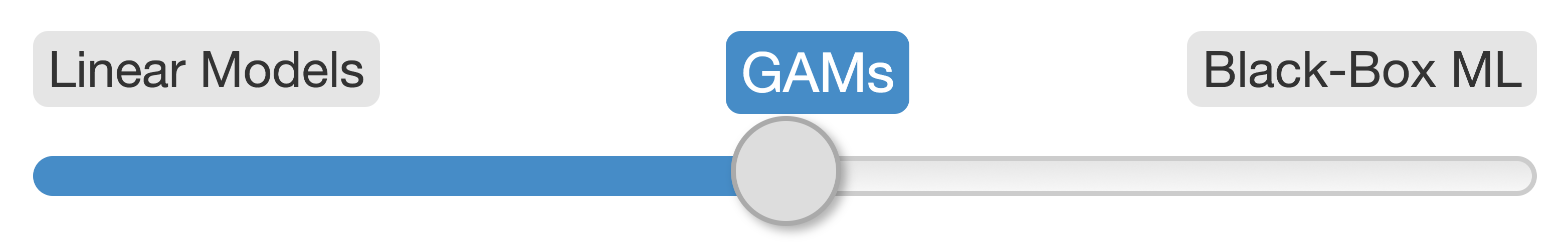 .references[Source: [GAMs in R by Noam Ross](https://noamross.github.io/gams-in-r-course/)] ??? GAMs are an intermediate-complexity model * can learn from data without needing to be informed by the user * remain interpretable because we can visualize the fitted features --- # How is a GAM different? `$$\begin{align*} y_i &\sim \mathcal{D}(\mu_i, \theta) \\ \mathbb{E}(y_i) &= \mu_i = g(\eta_i)^{-1} \end{align*}$$` We model the mean of data as a sum of linear terms: `$$\eta_i = \beta_0 +\sum_j \color{red}{ \beta_j x_{ji}}$$` A GAM is a sum of _smooth functions_ or _smooths_ `$$\eta_i = \beta_0 + \sum_j \color{red}{f_j(x_{ji})}$$` --- # How did `gam()` *know*? <!-- --> --- class: inverse background-image: url("./resources/rob-potter-398564.jpg") background-size: contain # What magic is this? .footnote[ <a style="background-color:black;color:white;text-decoration:none;padding:4px 6px;font-family:-apple-system, BlinkMacSystemFont, "San Francisco", "Helvetica Neue", Helvetica, Ubuntu, Roboto, Noto, "Segoe UI", Arial, sans-serif;font-size:12px;font-weight:bold;line-height:1.2;display:inline-block;border-radius:3px;" href="https://unsplash.com/@robpotter?utm_medium=referral&utm_campaign=photographer-credit&utm_content=creditBadge" target="_blank" rel="noopener noreferrer" title="Download free do whatever you want high-resolution photos from Rob Potter"><span style="display:inline-block;padding:2px 3px;"><svg xmlns="http://www.w3.org/2000/svg" style="height:12px;width:auto;position:relative;vertical-align:middle;top:-1px;fill:white;" viewBox="0 0 32 32"><title></title><path d="M20.8 18.1c0 2.7-2.2 4.8-4.8 4.8s-4.8-2.1-4.8-4.8c0-2.7 2.2-4.8 4.8-4.8 2.7.1 4.8 2.2 4.8 4.8zm11.2-7.4v14.9c0 2.3-1.9 4.3-4.3 4.3h-23.4c-2.4 0-4.3-1.9-4.3-4.3v-15c0-2.3 1.9-4.3 4.3-4.3h3.7l.8-2.3c.4-1.1 1.7-2 2.9-2h8.6c1.2 0 2.5.9 2.9 2l.8 2.4h3.7c2.4 0 4.3 1.9 4.3 4.3zm-8.6 7.5c0-4.1-3.3-7.5-7.5-7.5-4.1 0-7.5 3.4-7.5 7.5s3.3 7.5 7.5 7.5c4.2-.1 7.5-3.4 7.5-7.5z"></path></svg></span><span style="display:inline-block;padding:2px 3px;">Rob Potter</span></a> ] --- class: inverse background-image: url("resources/wiggly-things.png") background-size: contain --- # Fitting a GAM in R ```r model <- gam( y ~ s(x1) + s(x2) + te(x3, x4), # formula describing model data = my_data_frame, # your data method = "REML", # or "ML" family = gaussian # or something more exotic ) ``` `s()` terms are smooths of one or more variables `te()` terms are the smooth equivalent of *main effects + interactions* `$$\eta_i = \beta_0 + f(\mathtt{Year}_i)$$` ```r library("mgcv") gam(Temperature ~ s(Year, k = 10), data = gtemp, method = "REML") ``` --- class: middle center inverse subsection # Your turn --- # Exercise Complete the exercise at <https://gavinsimpson.github.io/physalia-gam-course/day-2/global-temperature.html> You can also download the [`global-temperature.qmd`](https://github.com/gavinsimpson/physalia-gam-course/raw/refs/heads/main/day-2/global-temperature.qmd) and open it in RStudio --- # Wiggly things .center[] ??? GAMs use splines to represent the non-linear relationships between covariates, here `x`, and the response variable on the `y` axis. --- # Basis expansions In the polynomial models we used a polynomial basis expansion of `\(\boldsymbol{x}\)` * `\(\boldsymbol{x}^0 = \boldsymbol{1}\)` — the model constant term * `\(\boldsymbol{x}^1 = \boldsymbol{x}\)` — linear term * `\(\boldsymbol{x}^2\)` * `\(\boldsymbol{x}^3\)` * … --- # Splines Splines are *functions* composed of simpler functions Simpler functions are *basis functions* & the set of basis functions is a *basis* When we model using splines, each basis function `\(b_k\)` has a coefficient `\(\beta_k\)` Resultant spline is a the sum of these weighted basis functions, evaluated at the values of `\(x\)` `$$s(x) = \sum_{k = 1}^K \beta_k b_k(x)$$` --- # Splines formed from basis functions <!-- --> ??? Splines are built up from basis functions Here I'm showing a cubic regression spline basis with 10 knots/functions We weight each basis function to get a spline. Here all the basisi functions have the same weight so they would fit a horizontal line --- # Weight basis functions ⇨ spline .center[] ??? But if we choose different weights we get more wiggly spline Each of the splines I showed you earlier are all generated from the same basis functions but using different weights --- # How do GAMs learn from data? <!-- --> ??? How does this help us learn from data? Here I'm showing a simulated data set, where the data are drawn from the orange functions, with noise. We want to learn the orange function from the data --- # Maximise penalised log-likelihood ⇨ β .center[] ??? Fitting a GAM involves finding the weights for the basis functions that produce a spline that fits the data best, subject to some constraints --- class: inverse middle center subsection # Avoid overfitting our sample --- class: inverse center middle large-subsection # How wiggly? $$ \int_{\mathbb{R}} [f^{\prime\prime}]^2 dx = \boldsymbol{\beta}^{\mathsf{T}}\mathbf{S}\boldsymbol{\beta} $$ --- class: inverse center middle large-subsection # Penalised fit $$ \mathcal{L}_p(\boldsymbol{\beta}) = \mathcal{L}(\boldsymbol{\beta}) - \frac{1}{2} \lambda\boldsymbol{\beta}^{\mathsf{T}}\mathbf{S}\boldsymbol{\beta} $$ --- # Wiggliness `$$\int_{\mathbb{R}} [f^{\prime\prime}]^2 dx = \boldsymbol{\beta}^{\mathsf{T}}\mathbf{S}\boldsymbol{\beta} = \large{W}$$` (Wiggliness is 100% the right mathy word) We penalize wiggliness to avoid overfitting --- # Making wiggliness matter `\(W\)` measures **wiggliness** (log) likelihood measures closeness to the data We use a **smoothing parameter** `\(\lambda\)` to define the trade-off, to find the spline coefficients `\(B_k\)` that maximize the **penalized** log-likelihood `$$\mathcal{L}_p = \log(\text{Likelihood}) - \lambda W$$` --- # HadCRUT4 time series <!-- --> --- # Picking the right wiggliness .pull-left[ Two ways to think about how to optimize `\(\lambda\)`: * Predictive: Minimize out-of-sample error * Bayesian: Put priors on our basis coefficients ] .pull-right[ Many methods: AIC, Mallow's `\(C_p\)`, GCV, ML, REML * **Practically**, use **REML**, because of numerical stability * Hence `gam(..., method="REML")` ] .center[  ] --- # Maximum allowed wiggliness We set **basis complexity** or "size" `\(k\)` This is _maximum wigglyness_, can be thought of as number of small functions that make up a curve Once smoothing is applied, curves have fewer **effective degrees of freedom (EDF)** EDF < `\(k\)` --- # Maximum allowed wiggliness `\(k\)` must be *large enough*, the `\(\lambda\)` penalty does the rest *Large enough* — space of functions representable by the basis includes the true function or a close approximation to the true function Bigger `\(k\)` increases computational cost In **mgcv**, default `\(k\)` values are arbitrary — after choosing the model terms, this is the key user choice **Must be checked!** — `k.check()` --- # GAM summary so far 1. GAMs give us a framework to model flexible nonlinear relationships 2. Use little functions (**basis functions**) to make big functions (**smooths**) 3. Use a **penalty** to trade off wiggliness/generality 4. Need to make sure your smooths are **wiggly enough** --- class: middle center inverse subsection # Your turn --- # Exercise Complete the exercise at <https://gavinsimpson.github.io/physalia-gam-course/day-2/milk-yield.html> You can also download the [`milk-yield.qmd`](https://github.com/gavinsimpson/physalia-gam-course/raw/refs/heads/main/day-2/milk-yield.qmd) and open it in RStudio --- class: middle center inverse subsection # Example --- # Portugese larks .row[ .col-7[ ``` r library("here"); library("readr"); library("dplyr") larks <- read_csv(here("data", "larks.csv"), col_types = "ccdddd") larks <- larks |> mutate(crestlark = factor(crestlark), linnet = factor(linnet), e = x / 1000, n = y / 1000) head(larks) ``` ``` ## # A tibble: 6 × 8 ## QUADRICULA TET crestlark linnet x y e n ## <chr> <chr> <fct> <fct> <dbl> <dbl> <dbl> <dbl> ## 1 NG56 E <NA> <NA> 551000 4669000 551 4669 ## 2 NG56 J <NA> <NA> 553000 4669000 553 4669 ## 3 NG56 P <NA> <NA> 555000 4669000 555 4669 ## 4 NG56 U <NA> <NA> 557000 4669000 557 4669 ## 5 NG56 Z <NA> <NA> 559000 4669000 559 4669 ## 6 NG66 E <NA> <NA> 561000 4669000 561 4669 ``` ] .col-5[ <!-- --> ] ] --- # Portugese larks — binomial GAM .row[ .col-6[ ``` r crest <- gam(crestlark ~ s(e, n, k = 100), data = larks, family = binomial, method = "REML") ``` `\(f(e, n)\)` indicated by `s(e, n)` in the formula Isotropic thin plate spline `k` sets size of basis dimension; upper limit on EDF Smoothness parameters estimated via REML ] .col-6[ .smaller[ ``` r summary(crest) ``` ``` ## ## Family: binomial ## Link function: logit ## ## Formula: ## crestlark ~ s(e, n, k = 100) ## ## Parametric coefficients: ## Estimate Std. Error z value Pr(>|z|) ## (Intercept) -2.24184 0.07785 -28.8 <2e-16 *** ## --- ## Signif. codes: 0 '***' 0.001 '**' 0.01 '*' 0.05 '.' 0.1 ' ' 1 ## ## Approximate significance of smooth terms: ## edf Ref.df Chi.sq p-value ## s(e,n) 74.04 86.46 857.3 <2e-16 *** ## --- ## Signif. codes: 0 '***' 0.001 '**' 0.01 '*' 0.05 '.' 0.1 ' ' 1 ## ## R-sq.(adj) = 0.234 Deviance explained = 25.9% ## -REML = 2499.8 Scale est. = 1 n = 6457 ``` ] ] ] --- # Portugese larks — binomial GAM Model checking with binary data is a pain — usual residuals look weird Alternatively, for some families, we can use Probability Integral Transform or Quantile residuals .pull-left[ .smaller[ ``` r residuals_linpred_plot(crest, type = "deviance") ``` <!-- --> ] ] .pull-right[ .smaller[ ``` r residuals_linpred_plot(crest, type = "quantile") ``` <!-- --> ] ] Also: DHARMa 📦 --- # Portugese larks — binomial GAM Alternatively we can aggregate data at the `QUADRICULA` level & fit a binomial count model .smaller[ ``` r larks2 <- larks |> mutate(crestlark = as.numeric(as.character(crestlark)), # to numeric linnet = as.numeric(as.character(linnet)), tet_n = rep(1, nrow(larks)), # counter for how many grid cells (tetrads) we sum N = rep(1, nrow(larks)), # number of observations, 1 per row currently N = if_else(is.na(crestlark), NA_real_, N)) |> # set N to NA if observation taken group_by(QUADRICULA) |> # group by the larger grid square summarise(across(c(N, crestlark, linnet, tet_n, e, n), ~ sum(., na.rm = TRUE))) |> # sum all needed variables mutate(e = e / tet_n, n = n / tet_n) # rescale to get avg E,N coords for QUADRICULA ## fit binomial GAM crest2 <- gam(cbind(crestlark, N - crestlark) ~ s(e, n, k = 100), data = larks2, family = binomial, method = "REML") ``` ] --- # Model checking .pull-left[ .smaller[ ``` r crest3 <- gam(cbind(crestlark, N - crestlark) ~ s(e, n, k = 100), data = larks2, family = quasibinomial, method = "REML") crest3$scale # should be == 1 ``` ``` ## [1] 1.729431 ``` ] Model residuals don't look too bad Bands of points due to integers Some overdispersion — φ = 1.73 ] .pull-right[ ``` r ggplot(tibble(Fitted = fitted(crest2), Resid = resid(crest2)), aes(Fitted, Resid)) + geom_point() ``` <!-- --> ] --- class: inverse middle center subsection # South Pole CO<sub>2</sub> --- # Atmospheric CO<sub>2</sub> ``` r library("gratia"); library("readr"); library("here") south <- read_csv(here("data", "south_pole.csv"), col_types = "ddd") south ``` ``` ## # A tibble: 507 × 3 ## co2 c.month month ## <dbl> <dbl> <dbl> ## 1 NA 1 1 ## 2 NA 2 2 ## 3 NA 3 3 ## 4 NA 4 4 ## 5 NA 5 5 ## 6 313. 6 6 ## 7 NA 7 7 ## 8 NA 8 8 ## 9 314. 9 9 ## 10 NA 10 10 ## # ℹ 497 more rows ``` --- # Atmospheric CO<sub>2</sub> ``` r ggplot(south, aes(x = c.month, y = co2)) + geom_line() ``` <img src="index_files/figure-html/co2-example-2-1.svg" width="95%" style="display: block; margin: auto;" /> --- # Atmospheric CO<sub>2</sub> — fit naive GAM .smaller[ ``` r m_co2 <- gam(co2 ~ s(c.month, k = 300, bs = "cr"), data = south, method = "REML") summary(m_co2) ``` ``` ## ## Family: gaussian ## Link function: identity ## ## Formula: ## co2 ~ s(c.month, k = 300, bs = "cr") ## ## Parametric coefficients: ## Estimate Std. Error t value Pr(>|t|) ## (Intercept) 3.382e+02 4.444e-03 76111 <2e-16 *** ## --- ## Signif. codes: 0 '***' 0.001 '**' 0.01 '*' 0.05 '.' 0.1 ' ' 1 ## ## Approximate significance of smooth terms: ## edf Ref.df F p-value ## s(c.month) 205.3 241.4 44646 <2e-16 *** ## --- ## Signif. codes: 0 '***' 0.001 '**' 0.01 '*' 0.05 '.' 0.1 ' ' 1 ## ## R-sq.(adj) = 1 Deviance explained = 100% ## -REML = 36.492 Scale est. = 0.0084334 n = 427 ``` ] --- # Atmospheric CO<sub>2</sub> — predict Predict the next 36 months ``` r new_df <- with(south, tibble(c.month = 1:(nrow(south) + 36))) fv <- fitted_values(m_co2, data = new_df, scale = "response") fv ``` ``` ## # A tibble: 543 × 6 ## .row c.month .fitted .se .lower_ci .upper_ci ## <int> <int> <dbl> <dbl> <dbl> <dbl> ## 1 1 1 312. 0.290 311. 313. ## 2 2 2 312. 0.247 312. 313. ## 3 3 3 312. 0.205 312. 313. ## 4 4 4 313. 0.164 312. 313. ## 5 5 5 313. 0.125 313. 313. ## 6 6 6 313. 0.0901 313. 313. ## 7 7 7 313. 0.0677 313. 314. ## 8 8 8 314. 0.0662 314. 314. ## 9 9 9 314. 0.0759 314. 314. ## 10 10 10 314. 0.0807 314. 314. ## # ℹ 533 more rows ``` --- # Atmospheric CO<sub>2</sub> — predict ``` r ggplot(fv, aes(x = c.month, y = .fitted)) + geom_ribbon(aes(ymin = .lower_ci, ymax = .upper_ci), alpha = 0.2) + geom_line(data = south, aes(c.month, co2), col = "red") + geom_line(alpha = 0.4) ``` <!-- --> --- # Atmospheric CO<sub>2</sub> — better model Decompose into 1. a seasonal smooth 2. a long term trend ``` r m2_co2 <- gam(co2 ~ s(month, bs = "cc") + s(c.month, bs = "cr", k = 300), data = south, method = "REML", knots = list(month = c(0.5, 12.5))) ``` --- # Atmospheric CO<sub>2</sub> — better model .smaller[ ``` r summary(m2_co2) ``` ``` ## ## Family: gaussian ## Link function: identity ## ## Formula: ## co2 ~ s(month, bs = "cc") + s(c.month, bs = "cr", k = 300) ## ## Parametric coefficients: ## Estimate Std. Error t value Pr(>|t|) ## (Intercept) 3.382e+02 5.331e-03 63447 <2e-16 *** ## --- ## Signif. codes: 0 '***' 0.001 '**' 0.01 '*' 0.05 '.' 0.1 ' ' 1 ## ## Approximate significance of smooth terms: ## edf Ref.df F p-value ## s(month) 7.266 8.0 165.1 <2e-16 *** ## s(c.month) 107.309 131.8 56450.2 <2e-16 *** ## --- ## Signif. codes: 0 '***' 0.001 '**' 0.01 '*' 0.05 '.' 0.1 ' ' 1 ## ## R-sq.(adj) = 1 Deviance explained = 100% ## -REML = -103.74 Scale est. = 0.012136 n = 427 ``` ] --- # Atmospheric CO<sub>2</sub> — predict ``` r nr <- nrow(south) new_df <- with(south, tibble(c.month = 1:(nr + 36), month = rep(seq_len(12), length = nr + 36))) fv2 <- fitted_values(m2_co2, data = new_df, scale = "response") fv2 ``` ``` ## # A tibble: 543 × 7 ## .row c.month month .fitted .se .lower_ci .upper_ci ## <int> <int> <int> <dbl> <dbl> <dbl> <dbl> ## 1 1 1 1 313. 0.296 312. 314. ## 2 2 2 2 313. 0.255 312. 313. ## 3 3 3 3 313. 0.214 312. 313. ## 4 4 4 4 313. 0.176 312. 313. ## 5 5 5 5 313. 0.137 313. 313. ## 6 6 6 6 313. 0.103 313. 313. ## 7 7 7 7 313. 0.0827 313. 314. ## 8 8 8 8 314. 0.0747 314. 314. ## 9 9 9 9 314. 0.0785 314. 314. ## 10 10 10 10 314. 0.0845 314. 314. ## # ℹ 533 more rows ``` --- # Atmospheric CO<sub>2</sub> — predict ``` r ggplot(fv2, aes(x = c.month, y = .fitted)) + geom_ribbon(aes(ymin = .lower_ci, ymax = .upper_ci), alpha = 0.2) + geom_line(data = south, aes(c.month, co2), col = "red") + geom_line(alpha = 0.4) ``` <!-- --> --- # A bestiary of conditional distributions A GAM is just a fancy GLM Simon Wood & colleagues (2016) have extended the *mgcv* methods to some non-exponential family distributions As of *mgcv* 📦 v 1.9.4: .small[ .row[ .col-5[ * `binomial()` * `poisson()` * `Gamma()` * `inverse.gaussian()` * `nb()` * `tw()` * `mvn()` * `multinom()` ] .col-4[ * `betar()` * `scat()` * `gaulss()` * `ziplss()` * `twlss()` * `cox.ph()` * `gevlss()` * `gamals()` ] .col-3[ * `ocat()` * `shash()` * `gumbls()` * `cnorm()` * `clog()` * `cpois()` * `ziP()` * `gfam()` * `bcg()` ] ] ] --- # A cornucopia of smooths The type of smoother is controlled by the `bs` argument (think *basis*) The default is a low-rank thin plate spline `bs = "tp"` Many others available .small[ .row[ .col-6[ * Cubic splines `bs = "cr"` * P splines `bs = "ps"` * Cyclic splines `bs = "cc"` or `bs = "cp"` * Adaptive splines `bs = "ad"` * Random effect `bs = "re"` * Factor smooths `bs = "fs"` ] .col-6[ * Duchon splines `bs = "ds"` * Spline on the sphere `bs = "sos"` * MRFs `bs = "mrf"` * Soap-film smooth `bs = "so"` * Gaussian process `bs = "gp"` * Constrained factor smooth `bs = "sz"` ] ] ] *mgcv* also provides shape constrained smooths (`bs = "sc"`), but can only be used in the new `scasm()` function --- # Thin plate splines Default spline in {mgcv} is `bs = "tp"` Thin plate splines — knot at every unique data value Penalty on wiggliness (default is 2nd derivative) As many basis functions as data This is wasteful --- # Low rank thin plate splines Thin plate regression spline Form the full TPS basis Take the wiggly basis functions and eigen-decomposition Concentrates the *information* in the TPS basis into as few as possible new basis functions Retain the `k` eigenvectors with the `k` largest eigenvalues as the new basis Fit the GAM with those new basis functions --- # Simulated Motorcycle Accident A data frame giving a series of measurements of head acceleration in a simulated motorcycle accident, used to test crash helmets ``` r library("dplyr"); library("ggplot2") data(mcycle, package = "MASS") mcycle <- as_tibble(mcycle) mcycle ``` ``` ## # A tibble: 133 × 2 ## times accel ## <dbl> <dbl> ## 1 2.4 0 ## 2 2.6 -1.3 ## 3 3.2 -2.7 ## 4 3.6 0 ## 5 4 -2.7 ## 6 6.2 -2.7 ## 7 6.6 -2.7 ## 8 6.8 -1.3 ## 9 7.8 -2.7 ## 10 8.2 -2.7 ## # ℹ 123 more rows ``` --- # Simulated Motorcycle Accident .row[ .col-6[ ``` r plt <- mcycle |> ggplot(aes(x = times, y = accel)) + geom_point() + labs(x = "Milliseconds after impact", y = expression(italic(g))) plt ``` ] .col-6[ <!-- --> ] ] --- # TPRS basis ``` r new_df <- with(mcycle, tibble(times = evenly(times, n = 100))) bfun <- basis(s(times), data = new_df) bfun ``` ``` ## # A tibble: 1,000 × 6 ## .smooth .type .by .bf .value times ## <chr> <chr> <chr> <fct> <dbl> <dbl> ## 1 s(times) TPRS <NA> 1 -1.60 2.4 ## 2 s(times) TPRS <NA> 2 -1.66 2.4 ## 3 s(times) TPRS <NA> 3 -1.84 2.4 ## 4 s(times) TPRS <NA> 4 -1.95 2.4 ## 5 s(times) TPRS <NA> 5 -1.98 2.4 ## 6 s(times) TPRS <NA> 6 2.08 2.4 ## 7 s(times) TPRS <NA> 7 2.06 2.4 ## 8 s(times) TPRS <NA> 8 -2.15 2.4 ## 9 s(times) TPRS <NA> 9 1 2.4 ## 10 s(times) TPRS <NA> 10 -1.71 2.4 ## # ℹ 990 more rows ``` --- # TPRS basis ``` r draw(bfun) ``` .center[ <img src="index_files/figure-html/draw-tprs-basis-1.svg" width="95%" /> ] --- # TPRS basis ``` r draw(bfun) + facet_wrap(~ .bf) ``` .center[ <img src="index_files/figure-html/draw-tprs-basis-facetted-1.svg" width="90%" /> ] --- # Cubic regression splines A CRS is composed of piecewise cubic polynomials over intervals of the data The intervals are defined by knots The individual cubic polynomials join at the knots so that resulting curve is continuous up to the second derivative In {mgcv} the knot location are at evenly-spaced *quantiles* of the covariate — not evenly through the data --- # Cubic regression splines ``` r bfun <- basis(s(times, bs = "cr"), data = new_df) draw(bfun) + facet_wrap(~ .bf) ``` <img src="index_files/figure-html/unnamed-chunk-3-1.svg" width="90%" style="display: block; margin: auto;" /> --- # Cubic regression splines <img src="index_files/figure-html/unnamed-chunk-4-1.svg" width="95%" style="display: block; margin: auto;" /> --- # Cubic regression splines Use can specify the knot locations using the `knots` argument to the `gam()` function `knots` takes a named list, with names equal to the covariate(s) you want to set the knot locations for ``` r ## how many basis functions? K <- 7 ## create the knots list knots <- with(mcycle, list(times = evenly(times, n = K))) ## provide `knots` to functions bfun <- basis(s(times, bs = "cr", k = K), data = new_df, knots = knots) model <- gam(accel ~ s(times, bs = "cr", k = K), data = mcycle, method = "REML", knots = knots) # <- specify knots to the model ``` --- # Cyclic cubic regression splines Cyclic cubic regression splines are CRS but with the additional constraint that curve is continuous to the 2nd derivative *at the end points of the data range* Specify the basis with `bs = "cc"` ``` r month_df <- with(south, tibble(month = evenly(month, n = 100))) bfun <- basis(s(month, bs = "cc"), data = month_df) ``` --- # Cyclic cubic regression splines ``` r draw(bfun) + facet_wrap(~ .bf) ``` <img src="index_files/figure-html/draw-crs-basis-facetted-1.svg" width="95%" style="display: block; margin: auto;" /> --- # Cyclic cubic regression splines A problem for `month` as we don't expect December & January to be *exactly* the same Set the outer knots ``` r knots <- list(month = c(0.5, 12.5)) bfun <- basis(s(month, bs = "cc"), data = month_df, knots = knots) draw(bfun) + facet_wrap(~ .bf) ``` --- # Cyclic cubic regression splines <!-- --> --- # The whole process 1 <!-- --> --- # The whole process 2 ``` r dat <- data_sim("eg1", seed = 4) m <- gam(y ~ s(x0) + s(x1) + s(x2, bs = "bs") + s(x3), data = dat, method = "REML") ``` ``` r draw(m, rug = FALSE) + plot_layout(nrow = 1, ncol = 4) ``` <!-- --> --- # The whole process 3 <!-- --> --- # Basis functions for `s(x, z)` Code for this is in `day-2/test.R` .center[ <img src="index_files/figure-html/tprs-2d-basis-1.svg" width="90%" /> ] --- # Basis functions for `s(x, z)` Panels 1–15 are the basis functions .center[ <img src="resources/wood-2ed-fig-5-12-2-d-tprs-basis-funs.png" width="45%" /> ] .small[ Source: Wood SN (2017) ] --- class: inverse middle center big-subsection # Penalties --- # How wiggly? $$ \int_{\mathbb{R}} [f^{\prime\prime}]^2 dx = \boldsymbol{\beta}^{\mathsf{T}}\mathbf{S}\boldsymbol{\beta} $$ `\(\mathbf{S}\)` is known as the penalty matrix Penalty matrix doesn't have to be derivative based — *P-splines* As long as we can write `\(\mathbf{S}\)` so that it measures the complexity of smooth as a function of the parameters of the smooth we're OK --- # TPRS basis ``` r new_df <- with(mcycle, tibble(times = evenly(times, n = 100))) bfun <- basis(s(times), data = new_df, constraints = TRUE) draw(bfun) + facet_wrap(~ .bf) ``` <img src="index_files/figure-html/unnamed-chunk-6-1.svg" width="85%" style="display: block; margin: auto;" /> --- # TPRS basis ``` r m <- gam(accel ~ s(times), dat = mcycle, method = "REML") S <- penalty(m, smooth = "s(times)") S ``` ``` ## # A tibble: 81 × 6 ## .smooth .type .penalty .row .col .value ## <chr> <chr> <chr> <chr> <chr> <dbl> ## 1 s(times) TPRS s(times) F1 F1 13.1 ## 2 s(times) TPRS s(times) F1 F2 2.71 ## 3 s(times) TPRS s(times) F1 F3 6.61 ## 4 s(times) TPRS s(times) F1 F4 2.05 ## 5 s(times) TPRS s(times) F1 F5 6.49 ## 6 s(times) TPRS s(times) F1 F6 -2.38 ## 7 s(times) TPRS s(times) F1 F7 7.97 ## 8 s(times) TPRS s(times) F1 F8 0.450 ## 9 s(times) TPRS s(times) F1 F9 0 ## 10 s(times) TPRS s(times) F2 F1 2.71 ## # ℹ 71 more rows ``` --- # TPRS basis & penalty .center[ <img src="index_files/figure-html/unnamed-chunk-8-1.png" width="100%" /> ] --- # CRS basis & penalty ``` r m <- gam(accel ~ s(times, bs = "cr"), data = mcycle, method = "REML") S <- penalty(m, smooth = "s(times)") # draw(S) ``` --- # CRS basis & penalty .center[ <img src="index_files/figure-html/unnamed-chunk-10-1.png" width="100%" /> ] --- class: inverse middle center big-subsection # gratia 📦 --- # gratia 📦 {gratia} is a package for working with GAMs Mostly limited to GAMs fitted with {mgcv} & {gamm4} Follows (sort of) Tidyverse principles * return tibbles (data frames) * suitable for plotting with {ggplot2} * graphics use {ggplot2} and {patchwork} --- # `draw()` The main function is `draw()` Has methods for many of the function outputs in {gratia} and for models --- # Plotting smooths ``` r m <- gam(accel ~ s(times), data = mcycle, method = "REML") draw(m) ``` <img src="index_files/figure-html/draw-mcycle-1.svg" width="90%" style="display: block; margin: auto;" /> --- # Plotting smooths ``` r df <- data_sim("eg1", n = 1000, seed = 42) df ``` ``` ## # A tibble: 1,000 × 10 ## y x0 x1 x2 x3 f f0 f1 f2 f3 ## <dbl> <dbl> <dbl> <dbl> <dbl> <dbl> <dbl> <dbl> <dbl> <dbl> ## 1 6.49 0.915 0.848 0.990 0.274 5.98 0.529 5.46 0.000000183 0 ## 2 4.32 0.937 0.0627 0.438 0.944 4.88 0.393 1.13 3.35 0 ## 3 6.17 0.286 0.820 0.700 0.446 9.62 1.57 5.15 2.90 0 ## 4 0.0454 0.830 0.539 0.889 0.542 4.06 1.02 2.94 0.102 0 ## 5 2.50 0.642 0.499 0.834 0.162 5.08 1.80 2.71 0.566 0 ## 6 6.13 0.519 0.0222 0.734 0.693 5.40 2.00 1.05 2.36 0 ## 7 7.50 0.737 0.554 0.647 0.797 7.80 1.47 3.03 3.30 0 ## 8 4.03 0.135 0.720 0.843 0.774 5.50 0.821 4.22 0.459 0 ## 9 8.95 0.657 0.236 0.160 0.213 10.5 1.76 1.60 7.15 0 ## 10 13.2 0.705 0.812 0.364 0.204 12.1 1.60 5.07 5.43 0 ## # ℹ 990 more rows ``` ``` r m_sim <- gam(y ~ s(x0) + s(x1) + s(x2) + s(x3), data = df, method = "REML") draw(m_sim) ``` --- # Plotting smooths .center[ <img src="index_files/figure-html/draw-four-fun-sim-plot-1.svg" width="95%" /> ] --- # Plotting smooths ``` r draw(m_sim, residuals = TRUE, # add partial residuals overall_uncertainty = TRUE, # include uncertainty due to constant unconditional = TRUE, # correct for smoothness selection rug = FALSE) # turn off rug plot ``` --- # Plotting smooths .center[ <img src="index_files/figure-html/draw-mcycle-options-plot-1.svg" width="95%" /> ]